What About Intra-Home Range Fix Density?
In a previous blog post I summarized an alternative approach to estimate local habitat selection, based on the individual’s characteristic scale of space use, CSSU, rather than local density of fixes (the utilization distibution, UD). In the present post I compare the density-based UD with local variation of CSSU in the context of habitat selection, using both simulated and real space use. Despite being critical to the traditional UD approach I also argue that density of fixes may still reveal important properties of value for ecological inference, and I describe this by an example.
In my book I argue strongly against using the traditional UD model as a proxy for strength of intra-home range habitat selection. The UD reflects local density of fixes. The reason for my critique is the UD’s intrinsically self-similar (fractal) structure under realistic home range conditions, while theoretical UD models are inherently non-fractal (“statistically smooth surface at fine resolutions”). The fractal property is expected to gradually emerge as the animal extends its familiarity with its habitat by tending to return to previously visited patches. In this process exploratory steps are intermingled with occasional returns to previous patches, leading to self-reinforcing strengthening of utilization of some patches on expense of others. In other words, this process describes positive feedback, which runs independently of local staying time per visit; i.e., return events add to the influence from environmental conditions per se since successive revisits are not independent events. The UD approach to estimate local selection strength depends on an assumption of independent revisits!
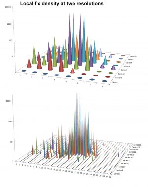 Below I describe the fractal (self-similar property of animal space use in a home range context, before comparing the UD approach and the alternative index for intra-home strength of habitat selection using real data. First, consider the set of simulated space use to the right. The data set is the same as the sample that was shown as a reference for serially non-autocorrelated fixes in this post. The spatially two-dimensional histogram (observe: log-transformed z-axes) illustrates the basic issue with the UD. When a virtual grid resolution is superimposed onto the scatter of fixes, the local density reflects a complex mixture of self-reinforcing patch use from directed return events, distance-from-centre effects and intra-patch density inflation from commuting between patches during return events. In addition, we have the influence from spatial scale to consider, since the model animal is utilizing its habitat in a multi-scaled manner. Thus, at finer grid resolutions the fixes become more aggregated within a subset of the grid cells, in a statistically non-trivial manner that violates basic model assumptions.
In the particular simulation above the environment was defined to be homogeneous. This homogeneity is implicit under the simplifying condition where return events to a previous location happens independently of the local habitat. This is of course unrealistic, but is applied in a modelling context for the purpose of disentangling intrinsic from extrinsic components of space use in a simplest possible manner. When the environment is homogeneous, local magnitude of CSSU is similar everywhere (despite the emergence of difference in local density of fixes; i.e., a non-trivially “jagged” UD). The tendency for spatial self-organization of fixes even in a homogeneous environment (intrinsically fractal dispersion, see below) may turn towards what has been termed “auto-facilitation”: local knowledge is gradually improving local patch value (e.g., foraging success) for the given individual, relative to similar patches that have not been visited (Gautestad and Mysterud 2010). In this manner an initially homogeneous environment from the perception of the animal will gradually become subjectively heterogeneous, due to the process of auto-facilitation.
A new animal of similar type and space use behaviour arriving in the same environment will have to build its own perception of its local conditions. In an a priori homogeneous environment the new animal’s UD will have the same over-all statistical properties like the magnitude of CSSU and fractal dimension (see below) but its fractal surface (local density variations of fixes) will be uncorrelated between the two individuals. As time goes by, also this individual may be expected to drift towards a subjective perception of a heterogeneous environment (the auto-facilitation effect). Despite the condition that these two individuals – in this thought example – are entering an a priori homogeneous environment, they are building respectively independent perceptions of environmental heterogeneity. On average, from superimposing many such subjective patch evaluations, brings us back to the homogeneous environment, because respective spatial representations are inter-individually independent (given that the added habitat value does not include a physical change of the respective patches).
If the habitat is a priori heterogeneous, the probability of returning to a given location is no longer a function of number of previous returns to this locations alone, but also influenced by a spatially varying reward expectation from returning. Thus, over time the homogeneous CSSU “field” that was described above may gradually turn towards a heterogeneous CSSU field that mirrors variations in local habitat selection strength. Smaller CSSU implies stronger space use intensity. Thus, 1/CSSU is a feasible expression for intensity. This extrinsic driver of adjustment to spatial heterogeneity – containing ecological information about local habitat selection intensity – requires specific procedures to be disentangled from the intrinsically driven heterogeneous dispersion of fix density that emerges even in a homogeneous environment. Local variation of 1/CSSU reflects the extrinsically driven strength of habitat selection, including physical patch manipulation if the auto-facilitation effect is not purely subjective. Please read this paragraph all over again, since this system property has frequently led to misconception of my Multi-scaled random walk (MRW) model and its statistical-mechanical framework.
 The illustration to the right shows how the fractal dimension of the scatter of fixes shown above may be estimated by counting number of non-empty grid cells (incidence, I) at varying grid resolutions, g. With log-transformed axes, a linear slope is expected if the pattern is fractal, and the dimension approximately equals the negative of the slope (in this example, D=1.03). The steeper slope at the coarsest resolutions (open symbols, D=2) is a statistical artifact, since splitting the arena in 2×2 and 4×4 cells does not resolve any “holes”; i.e., no cells are empty at these coarse resolutions when the arena size is the smallest rectangle that embeds all fixes.
What is the potential strength of the CSSU approach for applied ecology? Consider the following analysis of real data, where I compare intra-home range scores of local density of fixes of free-ranging sheep Ovis aries and local scores of the alternative index for local intensity of space use (the actual score is proportional with 1/C of the MRW model; i.e., 1/CSSU).
 In this pilot test the traditional density of fixes (open symbols) shows a weaker correlation with the actual soil fertility in the respective sub-sections of the home range, in comparison to the 1/CSSU index (filled symbols). The latter indicates a strong affinity to habitat patches that offered the best forage for the sheep. Low- and middle-quality areas had similar utilization intensity.
In my book I argue strongly against using the traditional UD model as a proxy for strength of intra-home range habitat selection. The UD reflects local density of fixes. The reason for my critique is the UD’s intrinsically self-similar (fractal) structure under realistic home range conditions, while theoretical UD models are inherently non-fractal (“statistically smooth surface at fine resolutions”). The fractal property is expected to gradually emerge as the animal extends its familiarity with its habitat by tending to return to previously visited patches. In this process exploratory steps are intermingled with occasional returns to previous patches, leading to self-reinforcing strengthening of utilization of some patches on expense of others. In other words, this process describes positive feedback, which runs independently of local staying time per visit; i.e., return events add to the influence from environmental conditions per se since successive revisits are not independent events. The UD approach to estimate local selection strength depends on an assumption of independent revisits!
In the particular simulation above the environment was defined to be homogeneous. This homogeneity is implicit under the simplifying condition where return events to a previous location happens independently of the local habitat. This is of course unrealistic, but is applied in a modelling context for the purpose of disentangling intrinsic from extrinsic components of space use in a simplest possible manner. When the environment is homogeneous, local magnitude of CSSU is similar everywhere (despite the emergence of difference in local density of fixes; i.e., a non-trivially “jagged” UD). The tendency for spatial self-organization of fixes even in a homogeneous environment (intrinsically fractal dispersion, see below) may turn towards what has been termed “auto-facilitation”: local knowledge is gradually improving local patch value (e.g., foraging success) for the given individual, relative to similar patches that have not been visited (Gautestad and Mysterud 2010). In this manner an initially homogeneous environment from the perception of the animal will gradually become subjectively heterogeneous, due to the process of auto-facilitation.
A new animal of similar type and space use behaviour arriving in the same environment will have to build its own perception of its local conditions. In an a priori homogeneous environment the new animal’s UD will have the same over-all statistical properties like the magnitude of CSSU and fractal dimension (see below) but its fractal surface (local density variations of fixes) will be uncorrelated between the two individuals. As time goes by, also this individual may be expected to drift towards a subjective perception of a heterogeneous environment (the auto-facilitation effect). Despite the condition that these two individuals – in this thought example – are entering an a priori homogeneous environment, they are building respectively independent perceptions of environmental heterogeneity. On average, from superimposing many such subjective patch evaluations, brings us back to the homogeneous environment, because respective spatial representations are inter-individually independent (given that the added habitat value does not include a physical change of the respective patches).
If the habitat is a priori heterogeneous, the probability of returning to a given location is no longer a function of number of previous returns to this locations alone, but also influenced by a spatially varying reward expectation from returning. Thus, over time the homogeneous CSSU “field” that was described above may gradually turn towards a heterogeneous CSSU field that mirrors variations in local habitat selection strength. Smaller CSSU implies stronger space use intensity. Thus, 1/CSSU is a feasible expression for intensity. This extrinsic driver of adjustment to spatial heterogeneity – containing ecological information about local habitat selection intensity – requires specific procedures to be disentangled from the intrinsically driven heterogeneous dispersion of fix density that emerges even in a homogeneous environment. Local variation of 1/CSSU reflects the extrinsically driven strength of habitat selection, including physical patch manipulation if the auto-facilitation effect is not purely subjective. Please read this paragraph all over again, since this system property has frequently led to misconception of my Multi-scaled random walk (MRW) model and its statistical-mechanical framework.
What is the potential strength of the CSSU approach for applied ecology? Consider the following analysis of real data, where I compare intra-home range scores of local density of fixes of free-ranging sheep Ovis aries and local scores of the alternative index for local intensity of space use (the actual score is proportional with 1/C of the MRW model; i.e., 1/CSSU).

The density index (local UD scores) is more fuzzy with respect to this relationship – a frustratingly common experience in use/availability analyses. For details on this analysis I refer to my book and to Gautestad (1998), Gautestad and Mysterud (2010).
I strongly encourage you to make a similar comparison using your own data when performing use/availability analyses.
So, what about local density? Does it have any significance for ecological inference at all in the present framework for complex space use? Yes, of course, but perhaps not in a manner you might have expected.
Generally, density of fixes is expected to be highest in localities close to the animal’s initial choice of spatial settlement. When the animal reaches a suitable habitat and is switching from a migratory to a sedentary mode (home range mode), the initial set of patches that the animal tends to return to will generate successively increasing peaks surrounding these localities in the UD. This tends to lead to a scale-free kind of self-reinforcing patch use, as already described. These local aggregations thus to some extent also reflect initial space use localities. If space use for some reason is drifting over time (Gautestad and Mysterud 2006), these aggregations become spatially dynamic and may be followed by splitting the time series of fixes into sub-periods. By studying the UD overlap (of lack thereof) from period to period one may infer about this behaviour and relate it to biological and ecological hypotheses.
In this manner, I propose that the UD has a great potential to reveal the animal’s initial settlement history, and – from this perspective – whether space use has been stable or drifting during the total period of fix sampling. However, as summarized above, the UD is expected to perform poorly in its traditional role, as a proxy for intra-home range habitat selection.
REFERENCES
Gautestad, A. O. 1998. The multiscaled home range. In: Site fidelity and scaling complexity in animal movement and habitat use: the multiscaled random walk model. Part 2: Scaling complexity in theory and practice. Dr. philos. thesis, University of Oslo. ISBN 82-90934-63-7.
Gautestad, A. O., and I. Mysterud. 2006. Complex animal distribution and abundance from memory-dependent kinetics. Ecological Complexity 3:44-55.
Gautestad, A. O., and I. Mysterud. 2010. Spatial memory, habitat auto-facilitation and the emergence of fractal home range patterns. Ecological Modelling 221:2741-2750.