Animal Space Use

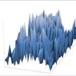
On rare occasions one’s research effort may lead to a Eureka! moment. While exploring and experimenting with the latest refinement of my Zoomer model for population dynamics I stumbled over a key condition to tune the model in and out of full coherence between spatial and temporal variability from the perspective of a self-similar statistical pattern. Fractal-like variability over space and time has been repeatedly reported in the ecological literature, but rarely has such pattern been studied simultaneously as two aspects of the same population. My hope is that the Zoomer model also has a more broadened potential by casting stronger light on the strange 1/f noise phenomenon (also called pink noise, or Flicker noise), which still tends to create paradoxes between empirical patterns and theoretical models in many fields of science. First, consider again some basic statistical aspects of a Zoomer-based simulation. Above I show the spatial dispersion of individuals within the given ar

In my continued quest for a more realistic statistical-mechanical theory for spatially extended population dynamics I have previously pointed out a specific property of the inter-scale spatial coefficient of variation as one of the hallmarks of scale-free dispersion (see Part III). In the present post I study another statistical property, the spatial autocorrelation, which may provide additional cue about the population’s compliance with standard or complex space use. First, consider the standard theory, based on mean field compliant population redistribution (mixing). The following three images show a typical example, where the population is subject to 5% diffusion rate at unit (pixel) scale, net population growth of 1%, no Allée effect, and over-all population density below carrying capacity. As previously described in this series and illustrated to the left, diffusion tends to smoothen the density surface. The log(M,V) plot over a scale range (below) typically shows y-interc

In the foregoing Part I suggested that the standard theoretical framework for simulating population dynamics/kinetics is fundamentally unrealistic, since in any open environment it dooms local population abundance to approaching zero and extinction due to memory-less dispersal and further lubricated by Allée effects. The only apparent rescue conditions for a population are (a) the population lives in a closed rather than open environment, which is an unrealistic scenario in general terms; or (b) on average the net growth rate is larger than the dispersal (diffusion) rate. In this post I argue that even the latter assumption is flawed. The traditional Coupled map lattice (CML) modelling, partial differential modelling, and other standard spin-offs from classical statistical mechanics may apparently be “rescued” with respect to model realism by defining unit spatial scale coarse enough to ensure that the net growth rate is stronger than diffusion rate at this level. Since diffusion is

Time to simulate a stress-test of the two population-kinetic frameworks, the traditional Coupled map lattice model and the novel Zoomer model! Consider a scenario where some kind of environmental event has crushed the population to about 1% of its normal carrying capacity. In addition, the remaining population has also become spatially fragmented during this catastrophe. Then consider that the condition improves to the pre-crash level. What is the population’s potential to recover under the two scenaria you have become familiar with in Parts I-IV, scale-specific and scale-free kinetics? The map to the right shows the small population’s spatial dispersion at the start of the potential recovery phase. Isopleths indicate local population density, which shows an average of 165 individuals pr. occupied cell at unit scale while the carrying capacity (CC) has been restored to a potential for 5,000 individuals at this scale. In other words, in this scenario most local populations have go

In the foregoing Parts I-III model complexity was increased in a stepwise manner for the sake of exploring intrinsic population behaviour one factor by the time. In this post I take one additional step by studying the overall statistical effect of environmental heterogeneity. For the time being I consider spatial heterogeneity only, leaving temporal fluctuations to a later post. Anyway, a new level of realism is hereby added relative to the scenaria in the previous posts: external influence is now adding to intrinsic processes with respect to variations in local population abundance. Consider the Zoomer snapshot to the right (zero diffusion, 5% zooming over a scale range, as in previous examples), after the population has progressed 100 time steps in an environment where the local carrying capacity varied over space (CC=2942 individuals pr. cell at unit scale within the arena, on average). Due to 50% overshoot survival (see Part I for a definition of CC), the population fluctuate