Analytical Sensitivity to Fuzzy Fix Coordinates
In empirical data GPS fixes are never exact positions. A “fuzziness field” will always be introduced due to uncertain geolocation. When analyzing a set of fixes in the context of multi-scaled space use, are the parameter estimates sensitive to this kind of statistical error? Simultaneously, I also explore the effect on constraining the potential home range by disallowing sallies to the outermost range of available area.
To explore the triangulation error effect on space use analysis I have simulated Multi-scaled random walk in a homogeneous environment with N=10,000 fixes (of which the first 1,000 fixes were discarded) under two scenaria; a “sharp” location (no uncertainty polygons), and strong fuzziness. The latter introduced a random displacement to each x-y coordinate with a standard deviation (SD) of magnitude approximately equal to the system condition’s Characteristic scale of space use (CSSU). Displacements to the outermost parts of the given arena was disallowed, to study how this may influence the analyses. I then ran the following three algorithms in the MRW Simulator: (a) analysis of A(N) at the home range scale, (b) analysis of A(N) at a local scale (splitting the home range into four quadrants), and (c) analysis of the fix scatters’ fractal property.
The following image shows the sharp fix set and the strongest fuzzyness condition.
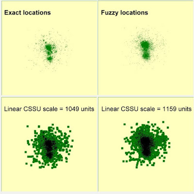
By visual inspection is is easy to spot the effect from the spatial error (SD = 1182 length units, upper row to the right). However, the respective A(N) analyses at the home range scale generated a CSSU estimate that was only 10% larger in the fuzzy set (linear scale). When superimposing cells of CSSU magnitude onto each fix, the home ranges appear quite similar in overall appearance and size. This was to be expected, since fuzziness influences fine-resolution space use only.
Visually, both home range areas appear somewhat constrained with respect to range, due to the condition to disallow displacements to the peripheral parts of the defined arena (influencing less than 1% of the displacements).
A(N) analysis (i.e., the Home range ghost formula; search Archive). The two conditions appeared quite similar in plots of log[I(N)], where I is the number of fix-embedding pixels at optimized pixel resolution, as described in previous posts.

However, for the fuzzy series there is a more pronounced break-point with a transition towards exponent ∼0.5 in sample size of magnitude larger than log2(N) ≈ 3. This break-point “lifted” the regression line somewhat for the fuzzy series, leading to a slightly larger intercept with the y-axis when interpolating towards log(N) = 0. This difference between the two conditions with respect to the y-intercept, Δlog(c) from the home range ghost formula log[I(N)] = log(c) + z*log(N), also defines the difference in CSSU when comparing sharp and fuzzy data sets. recall that CSSU ≡ c.
The spatial constraint on extreme displacements relative to the respective home ranges’ centres apparently did not influence these results.
 I have also superimposed local CSSU-analysis for respective four quadrants of the two home ranges. When area extent for analysis is constrained in this manner; i.e., spatial extent is reduced to 1:4 in area terms (1:2 linearly) for each local sub-set of fixes, respective (N,I) plot needs to be adjusted by a factor which compensates for the difference in scale range.
Since the present MRW conditions were run under fractal dimension D=1, each local log2[(N,I)] plot is rescaled to log2[(N,I)] + log2[ΔD(grain/extent)] = log2[(N,I)] + 1 when Δ regards the relative change of scale under condition D=1. After this rescaling the over-all CSSU and the local CSSU are overlapping, as shown by the regression lines in the A(N) analyses above. Overlapping CSSU implies that the four quadrants had similar space use conditions, which is true in this simplified case.
Fractal analysis. The Figure below shows the magnitude of incidence I as a function of relative spatial resolution k (the “box counting method”), spanning the scale range from k=1 (the entire arena, linear scale 40,000 units) and down to k = 40,000/(212) = 9.8 units, linear scale*.
 Starting from the coarsest resolution, k=1, the log-log regression obviously shows I = 1. At resolution k=1:2 and k=1:4 (4 and 16 grid cells, respectively), I = 4 and I = 4. In other words, all boxes contain fixes at k=1/2, apparently satisfying a two-dimensional object, and at k=1:4 some empty cells (12 of 16) are peeled away as empty space from the periphery of the fix scatter at this finer resolution.
This coarse-scale pattern is a consequence of the defined space use constraint. Disallowing “occasional sallies” outside the core home range obviously influences the number of non-empty boxes relative to all boxes available at the coarse resolutions 1< k < 4-1.
However, at progressively finer resolutions – below the “space fill effect” range transcending down to ca k=1:32 – the true fractal nature of the scatter of fixes begin to appear due to log-log linearity, confirming a statistical fractal with a stable dimension D≈1.1 over the resolution range 2-9 < k < 2-5 (showing log-log slope of -1.1). At finer resolutions, the dilution effect flattens further expansion of I. The D=1.1 scale range is close to expectation from the simulation conditions Dtrue=1, while the deviations above and below this range are trivial statistical artifacts from space filling and dilution.
The most interesting pattern regards the finest resolution range, where the fuzzy set of fixes somewhat unexpectedly follows a similar log(k,I) pattern as the non-fuzzy set. However, the slight difference in D, which increases to D =1.17, may be caused by the fuzziness (proportionally stronger space-fill effect as resolution is increased).
To conclude, if the magnitude of position uncertainty does not supersede the individual’s CSSU scale under the actual conditions, the A(N) analyses of MRW compliant space use does not seem to be seriously influenced by location fuzziness. The “fix scrambling” error is in most part subdued towards finer scales than the CSSU.
However, the story doesn’t end here. I have superimposed a dotted red line onto the Figure above. Overlapping with the D=1 section of grid resolutions, the line is extrapolated towards the intersection with log(I) ≈ 0 at a scale that is 21.5 = 2.8 times larger (linear) scale than the actual arena for the present analyses. In other words, in absence of area constraint and step length constraint (and disregarding step length constraint due to limited movement speed of the individual) one should expect the actual set of fixes to “fill up” the missing incidence over the coarse scale range, leading to D≈1 for the entire range from the dilution effect range towards coarser scales.
I have also marked the CSSU scale as the midpoint of the red line. A resolution of log2(k)=-5.5 is in fact very close to the CSSU estimate from the A(N) method (k=1:50 of actual arena using the A(N) method, versus 1:35 of the arena according to the fractal analysis). This alternative method to estimate CSSU was first published in this blog post.
A preliminary development towards this approach was explored both theoretically and empirically in Gautestad and Mysterud (2012).
NOTE
*) This analysis of N= 8,000 fixes, spanning box counting of 1, 2, 4, 16, 32, … 16.8 million grid cells at respective scales, took ca 10 hours pr. series in the MRW Simulator, using a laptop computer. I suppose this enormous number cracking it would be outside the practical range of a similar algorithm in R.
REFERENCES
Gautestad, A. O., and I. Mysterud. 2012. The Dilution Effect and the Space Fill Effect: Seeking to Offset Statistical Artifacts When Analyzing Animal Space Use from Telemetry Fixes. Ecological Complexity 9:33-42.
To explore the triangulation error effect on space use analysis I have simulated Multi-scaled random walk in a homogeneous environment with N=10,000 fixes (of which the first 1,000 fixes were discarded) under two scenaria; a “sharp” location (no uncertainty polygons), and strong fuzziness. The latter introduced a random displacement to each x-y coordinate with a standard deviation (SD) of magnitude approximately equal to the system condition’s Characteristic scale of space use (CSSU). Displacements to the outermost parts of the given arena was disallowed, to study how this may influence the analyses. I then ran the following three algorithms in the MRW Simulator: (a) analysis of A(N) at the home range scale, (b) analysis of A(N) at a local scale (splitting the home range into four quadrants), and (c) analysis of the fix scatters’ fractal property.
The following image shows the sharp fix set and the strongest fuzzyness condition.

By visual inspection is is easy to spot the effect from the spatial error (SD = 1182 length units, upper row to the right). However, the respective A(N) analyses at the home range scale generated a CSSU estimate that was only 10% larger in the fuzzy set (linear scale). When superimposing cells of CSSU magnitude onto each fix, the home ranges appear quite similar in overall appearance and size. This was to be expected, since fuzziness influences fine-resolution space use only.
Visually, both home range areas appear somewhat constrained with respect to range, due to the condition to disallow displacements to the peripheral parts of the defined arena (influencing less than 1% of the displacements).
A(N) analysis (i.e., the Home range ghost formula; search Archive). The two conditions appeared quite similar in plots of log[I(N)], where I is the number of fix-embedding pixels at optimized pixel resolution, as described in previous posts.

However, for the fuzzy series there is a more pronounced break-point with a transition towards exponent ∼0.5 in sample size of magnitude larger than log2(N) ≈ 3. This break-point “lifted” the regression line somewhat for the fuzzy series, leading to a slightly larger intercept with the y-axis when interpolating towards log(N) = 0. This difference between the two conditions with respect to the y-intercept, Δlog(c) from the home range ghost formula log[I(N)] = log(c) + z*log(N), also defines the difference in CSSU when comparing sharp and fuzzy data sets. recall that CSSU ≡ c.
The spatial constraint on extreme displacements relative to the respective home ranges’ centres apparently did not influence these results.
Since the present MRW conditions were run under fractal dimension D=1, each local log2[(N,I)] plot is rescaled to log2[(N,I)] + log2[ΔD(grain/extent)] = log2[(N,I)] + 1 when Δ regards the relative change of scale under condition D=1. After this rescaling the over-all CSSU and the local CSSU are overlapping, as shown by the regression lines in the A(N) analyses above. Overlapping CSSU implies that the four quadrants had similar space use conditions, which is true in this simplified case.
Fractal analysis. The Figure below shows the magnitude of incidence I as a function of relative spatial resolution k (the “box counting method”), spanning the scale range from k=1 (the entire arena, linear scale 40,000 units) and down to k = 40,000/(212) = 9.8 units, linear scale*.

This coarse-scale pattern is a consequence of the defined space use constraint. Disallowing “occasional sallies” outside the core home range obviously influences the number of non-empty boxes relative to all boxes available at the coarse resolutions 1< k < 4-1.
However, at progressively finer resolutions – below the “space fill effect” range transcending down to ca k=1:32 – the true fractal nature of the scatter of fixes begin to appear due to log-log linearity, confirming a statistical fractal with a stable dimension D≈1.1 over the resolution range 2-9 < k < 2-5 (showing log-log slope of -1.1). At finer resolutions, the dilution effect flattens further expansion of I. The D=1.1 scale range is close to expectation from the simulation conditions Dtrue=1, while the deviations above and below this range are trivial statistical artifacts from space filling and dilution.
The most interesting pattern regards the finest resolution range, where the fuzzy set of fixes somewhat unexpectedly follows a similar log(k,I) pattern as the non-fuzzy set. However, the slight difference in D, which increases to D =1.17, may be caused by the fuzziness (proportionally stronger space-fill effect as resolution is increased).
To conclude, if the magnitude of position uncertainty does not supersede the individual’s CSSU scale under the actual conditions, the A(N) analyses of MRW compliant space use does not seem to be seriously influenced by location fuzziness. The “fix scrambling” error is in most part subdued towards finer scales than the CSSU.
However, the story doesn’t end here. I have superimposed a dotted red line onto the Figure above. Overlapping with the D=1 section of grid resolutions, the line is extrapolated towards the intersection with log(I) ≈ 0 at a scale that is 21.5 = 2.8 times larger (linear) scale than the actual arena for the present analyses. In other words, in absence of area constraint and step length constraint (and disregarding step length constraint due to limited movement speed of the individual) one should expect the actual set of fixes to “fill up” the missing incidence over the coarse scale range, leading to D≈1 for the entire range from the dilution effect range towards coarser scales.
I have also marked the CSSU scale as the midpoint of the red line. A resolution of log2(k)=-5.5 is in fact very close to the CSSU estimate from the A(N) method (k=1:50 of actual arena using the A(N) method, versus 1:35 of the arena according to the fractal analysis). This alternative method to estimate CSSU was first published in this blog post.
A preliminary development towards this approach was explored both theoretically and empirically in Gautestad and Mysterud (2012).
NOTE
*) This analysis of N= 8,000 fixes, spanning box counting of 1, 2, 4, 16, 32, … 16.8 million grid cells at respective scales, took ca 10 hours pr. series in the MRW Simulator, using a laptop computer. I suppose this enormous number cracking it would be outside the practical range of a similar algorithm in R.
REFERENCES
Gautestad, A. O., and I. Mysterud. 2012. The Dilution Effect and the Space Fill Effect: Seeking to Offset Statistical Artifacts When Analyzing Animal Space Use from Telemetry Fixes. Ecological Complexity 9:33-42.