Parallel Processing – How to Verify It
In my previous post I contrasted the qualitative difference between animal space use under parallel processing (PP) and the standard, mechanistic approach. In this post I take the illustration one step further by illustrating how PP – in contrast to the mechanistic approach – allows for the simultaneous execution of responses and goals at different time scales. This architecture is substantially different from the traditional mechanistic models, which are locked into a serial processing kind of dynamics. This crucial difference in modelling dynamics allows for a simple statistical test to differentiate between true scale-free movement and look-alike variants; for example, composite random walk that is fine-tuned towards producing apparently scale-free movement.
First, recall that I make a clear distinction between a mechanistic model and a dynamic model. The former is a special case of a dynamic model, which is broader in scope by including true scale-free processing; i.e., PP. In my previous post I rolled dice to explain the difference.
In the traditional framework there is no need to distinguish between a mechanistic and a dynamic evolution, simply because in this special case of dynamics time pr. definition is one-dimensional. On the other hand, in the PP framework time is generally two-dimensional to allow for parallel execution of a process (for example, movement) at different scales at any moment in time.
Ignoring this biophysical distinction has over the years produced a lot of unnecessary confusion and misinterpretation with respect to the Multi-scaled random walk model (MRW), which is dynamic but non-mechanistic. The distinction apparently sounds paradoxical in the standard modelling world, but not in the PP world. I say it again: MRW is non-mechanistic, non-mechanistic, non-mechanistic – but still dynamic!
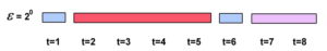 First, consider multi-scale movement in the comfort zone of mechanistic models. You may also call it serial processing, or Markov compliant. In the image to the right we see a (one-dimensional) time progression over a time span t=1,….,8 of a series where unit time scale per definition equals one (ε = 1; see my previous post). Some sequences are processed at a coarser scale than unit scale; for example, during the interval from t=2 to t=5 the animal “related to” its environment in a particularly coarse-scaled manner relative to unit time. Consider an area-restricted search (ARS) scenario, where the unit-scale moves (light blue events) regard temporally more high-frequency search within a local food patch and more coarse-scaled moves regard temporally toggling into a mode of more inter-patch movement. Consider that the animal during this time temporarily switched to a behavioural mode whereby environmental input is less direction- and speed-influencing (as seen from the unit scale) than during intra-patch search.
Within a mechanistic framework, processing at different scales (temporal resolutions) cannot take place simultaneously. The process needs to toggle (Gautestad 2011), as illustrated above.
Mechanistically, the ARS scenario is often parsimoniously modelled by a composite, correlated random walk. By fine-tuning the model parameters an the relative frequencies of toggling it has been shown how such a pattern may even produce approximately scale-free distribution of displacements; i.e, Lévy-like movement (Benhamou 2007). Such statistical similarity between two distinct dynamical classes has produced much fuzz in the field of animal movement research.
 Next, contrast the Lévy look-alike model above with a true scale-free process to the right. Due to the dynamics being executed over a continuum of temporal scales, we get a hierarchical structure of events. Thanks to the extra ε axis, there is no intrinsic paradox – as in a mechanistic system – due to a mixture of simultaneous events at different resolutions. Again, I refer to my previous “rolling dice” description. Despite a potential for fine-tuning the composite random walk model to look statistically scale-free, this mechanistic variant and the dynamically scale-free Lévy walk belongs to different corners of the Scaling cube.
Finally, how to distinguish a PP compliant kind of scale-free dynamics from the look-alike process? Coarse-grain the time series and see if the scale-free property persists or not (Gautestad 2013)!

The simulation above of a two-level Brownian motion model was performed under four conditions of ratio lambda between the scale parameter of the respective levels, lambda2/lambda1, where frequency of execution t2/t1 = 10 under all conditions. For each condition of lambda the simulated series were sampled at three time scales (lags, tobs); first using every step, then sampling 1:10 and then sampling 1:100. Original series lengths were increased proportionally in order to maintain the same sample size under each sampling scheme (20 000 steps). A double-log scatter plot (logarithmic base 2) of step length frequency, log(F), as a function of binned step length, log(L), was then made for each of the four parameter conditions and each of the three sampling schemes. Part (a): The result from lambda = 4 shows a linear regression slope and thus power law compliance over some part of the tail part of the distribution, with slope b = 2.9; i.e. the transition zone between Lévy walk (1 < b < 3) and Brownian motion (b >= 3 and increasing with increasing L, leading to steeper slope). At coarser time scales tobs = 10 and tobs = 100 the pattern is transformed to a generic-looking Brownian motion with exponential tail, which becomes linear in a semi-log plot: the inset shows the pattern from tobs = 100. Part (b): The results from lambda = 8.
Both the step length distribution (above) and the visual inspection of the path at different temporal scales reveal the true nature of the model: a look-alike scale-free and pseudo-Lévy pattern when the data are studied at unit scale where the fine-tuning of the parameters were performed, but shape-shifting towards the standard (mechanistic) random walk at coarser scales. A true PP-compliant process; i.e., non-mechanistic, would have maintained the Lévy pattern even at different sampling scales (Gautestad 2012).

Above: simulated paths of two-scale Brownian motion where 1000 steps are collected at time intervals 1:1, 1:10 and 1:100 relative to unit scale for the simulation, with lambda2/lambda1 = 15. The pattern shifts gradually from Lévy walk-like towards Brownian motion-like with increasing temporal scale relative to the execution scale (t = 1) for the simulations. Since the number of observations is kept constant the spatial extent of the path is increasing with increasing interval.
By the way, the PP conjecture also extends to the MRW-complementary population dynamical expression of animal space use, the Zoomer model (search Archive). This property can be clearly seen in the Zoomer model’s mathematical expression.
REFERENCES
Benhamou, S. 2007. How many animals really do the Lévy walk? Ecology 88:1962-1969.
Gautestad, A. O. 2011. Memory matters: Influence from a cognitive map on animal space use. Journal of Theoretical Biology 287:26-36.
Gautestad, A. O. 2012. Brownian motion or Lévy walk? Stepping towards an extended statistical mechanics for animal locomotion. Journal of the Royal Society Interface 9:2332-2340.
Gautestad, A. O. 2013. Animal space use: Distinguishing a two-level superposition of scale-specific walks from scale-free Lévy walk. Oikos 122:612-620.
First, recall that I make a clear distinction between a mechanistic model and a dynamic model. The former is a special case of a dynamic model, which is broader in scope by including true scale-free processing; i.e., PP. In my previous post I rolled dice to explain the difference.
In the traditional framework there is no need to distinguish between a mechanistic and a dynamic evolution, simply because in this special case of dynamics time pr. definition is one-dimensional. On the other hand, in the PP framework time is generally two-dimensional to allow for parallel execution of a process (for example, movement) at different scales at any moment in time.
Ignoring this biophysical distinction has over the years produced a lot of unnecessary confusion and misinterpretation with respect to the Multi-scaled random walk model (MRW), which is dynamic but non-mechanistic. The distinction apparently sounds paradoxical in the standard modelling world, but not in the PP world. I say it again: MRW is non-mechanistic, non-mechanistic, non-mechanistic – but still dynamic!
Within a mechanistic framework, processing at different scales (temporal resolutions) cannot take place simultaneously. The process needs to toggle (Gautestad 2011), as illustrated above.
Mechanistically, the ARS scenario is often parsimoniously modelled by a composite, correlated random walk. By fine-tuning the model parameters an the relative frequencies of toggling it has been shown how such a pattern may even produce approximately scale-free distribution of displacements; i.e, Lévy-like movement (Benhamou 2007). Such statistical similarity between two distinct dynamical classes has produced much fuzz in the field of animal movement research.
Finally, how to distinguish a PP compliant kind of scale-free dynamics from the look-alike process? Coarse-grain the time series and see if the scale-free property persists or not (Gautestad 2013)!

The simulation above of a two-level Brownian motion model was performed under four conditions of ratio lambda between the scale parameter of the respective levels, lambda2/lambda1, where frequency of execution t2/t1 = 10 under all conditions. For each condition of lambda the simulated series were sampled at three time scales (lags, tobs); first using every step, then sampling 1:10 and then sampling 1:100. Original series lengths were increased proportionally in order to maintain the same sample size under each sampling scheme (20 000 steps). A double-log scatter plot (logarithmic base 2) of step length frequency, log(F), as a function of binned step length, log(L), was then made for each of the four parameter conditions and each of the three sampling schemes. Part (a): The result from lambda = 4 shows a linear regression slope and thus power law compliance over some part of the tail part of the distribution, with slope b = 2.9; i.e. the transition zone between Lévy walk (1 < b < 3) and Brownian motion (b >= 3 and increasing with increasing L, leading to steeper slope). At coarser time scales tobs = 10 and tobs = 100 the pattern is transformed to a generic-looking Brownian motion with exponential tail, which becomes linear in a semi-log plot: the inset shows the pattern from tobs = 100. Part (b): The results from lambda = 8.
Both the step length distribution (above) and the visual inspection of the path at different temporal scales reveal the true nature of the model: a look-alike scale-free and pseudo-Lévy pattern when the data are studied at unit scale where the fine-tuning of the parameters were performed, but shape-shifting towards the standard (mechanistic) random walk at coarser scales. A true PP-compliant process; i.e., non-mechanistic, would have maintained the Lévy pattern even at different sampling scales (Gautestad 2012).

Above: simulated paths of two-scale Brownian motion where 1000 steps are collected at time intervals 1:1, 1:10 and 1:100 relative to unit scale for the simulation, with lambda2/lambda1 = 15. The pattern shifts gradually from Lévy walk-like towards Brownian motion-like with increasing temporal scale relative to the execution scale (t = 1) for the simulations. Since the number of observations is kept constant the spatial extent of the path is increasing with increasing interval.
By the way, the PP conjecture also extends to the MRW-complementary population dynamical expression of animal space use, the Zoomer model (search Archive). This property can be clearly seen in the Zoomer model’s mathematical expression.
REFERENCES
Benhamou, S. 2007. How many animals really do the Lévy walk? Ecology 88:1962-1969.
Gautestad, A. O. 2011. Memory matters: Influence from a cognitive map on animal space use. Journal of Theoretical Biology 287:26-36.
Gautestad, A. O. 2012. Brownian motion or Lévy walk? Stepping towards an extended statistical mechanics for animal locomotion. Journal of the Royal Society Interface 9:2332-2340.
Gautestad, A. O. 2013. Animal space use: Distinguishing a two-level superposition of scale-specific walks from scale-free Lévy walk. Oikos 122:612-620.