Post no. 100: Further support of the "infinite home range size" paradox
Memory map utilization by animals has received increased focus by behavioural ecologists. However, statistical and dynamic models in this field are in my view seriously lagging behind, as they are generally firmly glued to statistical-mechanical principles that defy the effects of realistic memory utilization. Consequently, several statistical paradoxes haunt the classical modelling framework, due to unrealistic model assumptions. An alternative statistical-physical approach is required altogether. In this post I illustrate one specific space use property that emerges under the alternative model, the "infinitely expanding home range size" as a function of observation intensity. Paradox resolved, and practical applications offered! The current example underscores how this alternative framework may be applied in ecological analysis of animal space use and habitat selection.
Struggling to define "home range size" or "outlier fixes" from your GPS series? What about problems with serial autocorrelation? Under the alternative model these issues find a logical solution.
Consider simulating GPS fixes from the generic model approach under the non-standard framework: Multi-scaled Random Walk (MRW), where the model animal move around in accordance to three main principles: (a) it occasionally returns to a previous location, (b) it relates to its environment in a scale-free manner, and (c) the latter aspect builds on a conjecture of parallel processing (i.e., a non-Markovian process; search this blog for all thee aspects).
For example, MRW highlights an apparent paradox of "infinitely expanding home range size", opposing the paradigm of an area asymptote as a set of N relocations (fixes) are increased. Seen from the sideline, the traditional expectation is that a set of serially non-autocorrelated fixes is expected to show an asymptotic approach towards the true home range as N grows. In other words, "missing area" is expected to be a small-sample artifact, to be counteracted by a larger N or accounted for by paradigm-compliant home range estimation models like Brownian bridge, KDE and many others. Serially autocorrelated fixes are also subject to similar analyses, but with some model adjustments or some simplifying assumptions.
However, all these standard approaches rest on some specific (often hidden or ignored) statistical assumptions about the animal's movement behaviour related to cognitive capacity to utilize memory. An alternative approach to resolve these issues is nutshell-explained below. For a deeper introduction I refer to my blog, book and papers.
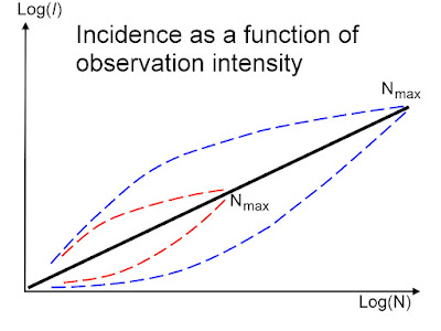
Consider the illustration of MRW below, where individual space use is calculated from N fixes, and area regards the number of "tiles" - incidence, I, embedding one or more fixes, at a specific grid resolution (tile size, or "system grain").
The default expectation, based on ideally non-autocorrelated fixes, is shown as a thick black line: I(N) = cN0.5, where c may be normalized to unit size to simplify the illustration: log(c) = 0 for N = 1. Under log transformation this means a line with slope 0.5 starting at the origin; i.e., log(area) expanding proportionally with 0.5*log(N), as shown by the thick black line.
Alternatively, based on serially autocorrelated fixes in MRW simulations, the coloured, dotted lines in the illustration reveals the property of "infinite area expansion", by showing log(I) over the given range from N=1 to total series length, Nmax.
Consider the first set of fixes (red, dotted lines), where I increases towards Nmax as sample size is expanded from two protocols; constant time interval, t, between successive fixes (continuous sampling up to total time T=Nt), or reduction of time interval as N is approaching Nmax within a fixed T (increased sampling frequency within T). The evolution of I from continuous sampling is illustrated by the lower red line, and frequency sampling by the upper line. In short, the latter (logically) reveals a smaller I for e given N, relative to the increased frequency sampling. However both methods (logically) end up at the same log(I) at the point Nmax.
Next, consider the same condition of autocorrelated fixes but using a larger Nmax, shown by the blue lines. Under the default condition of non-autocorrelated fixes, both sampling schemes are expected to fall on the same thick black line, confirming I(Nmax) increasing proportionally with 0.5*(Nmax). However, under the condition of autocorrelated fixes the blue lines from the two sub-sampling protocols diverge, as shown.
Obviously, the apparent slow-down of I(N) in the upper red line under the autocorrelation condition is not a symptom of an area asymptote, as proved by the upper blue line from an expanded data set. These patterns show false area asymptotes!
Observe that averaging the log(I) results from the two protocols and taking the log-average (taking the "geometric mean") brings the result in compliance with a slope 0.5; i.e., neatly falling on the thick black line! Hence, observation intensity, N, and not time as such (T or t) determines observed space use.
Collecting fix samples with short intervals or environmental perturbations of space use (drifting site fidelity) leads to autocorrelation. In short, if fix sampling interval is too short to embed several memory-based return events on average, or if the animal has partly or fully shifted its site fidelity pattern, the fixes are expected to become serially autocorrelated. Recently, I explored MRW's behaviour under the the latter scenario of drifting site fidelity (Gautestad 2022).
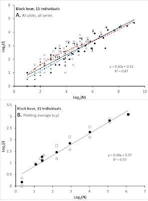
In this paper you also find a re-analysis of black bear Ursus americanus data applying our I(N) method as outlined above, confirming previous results using an alternative statistical method (Gautestad et al. 1998). I reproduce one of the Figures from Gautestad (2022) here*.
In short, the results again lend strong support to the hypothesis that these individuals followed a Multi-scaled Random Walk (MRW) kind of memory-influenced scale-free space use; i.e., PP compliant!
Thus, at this stage it should be safe to challenge researchers to try out the alternative approach to animal space use analysis based on GPS data.
- Accept the premise that the individual(s) adhere(s) to the PP conjecture; i.e., following the principles of scale-free movement and site fidelity under a cognitive capacity of patio-temporal memory utilization**. in other words, one expects a qualitatively very different kind of GPS fix dispersion relative to the traditional expectation from patterns that are generated from a Markov-compliant process (please search this blog, or read my book).
- Apply the respective estimates of non-normalized c, which is termed "Characteristic Scale of Space Use" (CSSU), as a proxy for the individual's relative strength of habitat selection within the given space extent and time period.
- Study the behaviour of CSSU under smaller sub-sections of the area, or under subsections of sampling period, to get indications of local and temporal variations of habitat selection.
Why not fight the hill of ignorance that is generated by the temptation to look another way when new theoretical approaches are challenging your beliefs at a deep level? I end this Blog post number 100 by citing Socrates:
NOTES
* Figure legend: (A) Results of re-analysis fixes from a sample of 15 telemetry series of black bear, where N-dependency for respective series is analyzed by I(N) rather than rescaled range analysis R/S [see Gautestad (2022)]. Plots of log2[I(N)] for time-continuous (diamonds), frequency-distributed sampling (squares) and the log-average of the two schemes (black circles) shows compliance with power exponent z~0.5 for the latter (continuous line). All sets from all schemes are superimposed, which implies a mixture of series with different Nmax. The slight non-linearity of time-continuous and frequency-distributed sampling is visualized by curve-fitting by third order polynomials (blue and red dashed lines, respectively). (B) The divergence between the two fix sampling schemes over the mid-range of N is better visualized by averaging over respective series’ I(N)-plots.
** You should make your own tests this conjecture by applying the protocols that has ben described repeatedly in my book, papers, and in this blog.
REFERENCES
Gautestad, A. O. 2015. Animal Space Use: Memory Effects, Scaling Complexity, and Biophysical Model Coherence Dog Ear Publishing, Indianapolis.
Gautestad, A. O. 2021. Animal Space Use, Second Edition: Memory Effects, Scaling Complexity and Biophysical Model Coherence. Cambridge Scholars Publishing, Newcastle upon Tyne.
Gautestad, A. O. 2022. Individual Network Topology of Patch Selection Under Influence of Drifting Site Fidelity. Frontiers in Ecology and Evolution 10:695854.
Gautestad, A. O., I. Mysterud, and M. R. Pelton. 1998. Complex movement and scale-free habitat use: testing the multi-scaled home range model on black bear telemetry data. Ursus 10:219-234.


