A Statistical-Mechanical Perspective on Site Fidelity – Part VI
In Part III of this group of posts I described how to estimate an animal’s characteristic scale of space use, CSSU, by zooming over a range of pixel resolutions until “focus” is achieved according to the Home range ghost function I(N)=c√N. This pixel size regards the balancing point where observed inward contraction of entropy equals outward expansion of entropy, as sample size of fixes N is changed. If the power exponent satisfies 0.5 [i.e., square root expansion of I(N)], the MRW theory states that the animal – in statistical terms – had put equal weight into habitat utilization over the actual scale range of space use. In Part V I explained two new statistical-mechanical concepts, micro-and macrostates of a system, but in the context of the classical framework. In this follow-up post I’m approaching the behaviour of these key properties under the condition of complex space use, both at the “balancing scale” CSSU and by zooming over its surrounding range of scales. In other words, while the CSSU property from an I(N) regression was studied with respect to observational intensity, N, at a given spatial scale, I here describe the system at different spatial scales at a given N.
First, a summary of the standard framework. As explained in Part II in this group of posts, in a classic statistical-mechanical system in the ergodic state (non-autocorrelated fixes, in the context of a home range) there is no “surprise factor” when we are observing the system at different spatial scales. In short, the total entropy is not influenced by our observational scale. For example, if we superimpose a virtual grid upon a set of “classically distributed” GPS fixes (i.e., in compliance with the convection model for the home range-generating process) and observe the system in its ergodic state, the total entropy depends only on the spatial extent, not on the choice of grid resolution (unless the sample of fixes is serially autocorrelated, as described in another post). In the equilibrium state, the entropy for the home range equals the sum of entropy in respective grid cells multiplied with a trivial conversion factor to compensate for difference in resolution, whether we choose to study the system from a fine or coarse spatial resolution.
This property of a classically derived statistical mechanics explains why in this branch of physics – the classic Boltzmann-Gibbs statistical mechanics – you won’t find any reference to an “observer effect” on entropy from zooming over pixel scales.
Translating this standard statistical-mechanical framework to a more familiar context of statistical ecology, the sum of grid cell variance equals the total variance of the system, quite independent of the grid resolution. The variance is thus reflecting a statistically stationary space use process. Consequently, in this classical scenario stationary variance (and entropy) supports the prediction of a home range area asymptote; a stationary home range size that will be revealed in more detail as N is sufficiently increased to reduce the statistical artifact from a small sample size. For larger N, home range area is practically constant under a change of N. Hence, the embedded entropy is similarly constant. In this manner I have hereby described a bridge between statistical ecology and statistical physics under the standard framework.
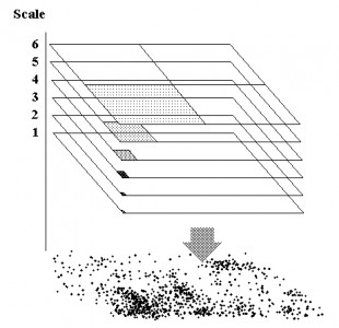 However, more bridge-building is needed, in particular with respect to complex animal space use. In the illustration to the left (copied from Gautestad et al. 1998) I have indicated a geometric scaling of a virtual grid that is superimposed upon a set of GPS fixes; cells scale by a power of 2 in this “sandwich” of resolutions. The choice to use power of 2 means that the respective resolutions’ cell areas scale by a factor of 4 (from top level towards finer resolutions: 1, 1/4, 1/16, 1/64, etc). This geometric scaling has a purpose, because it illustrates how a multi-scaled process – “complex space use” – is postulated to scale in a similarly geometric manner.
One may call it remarkable or fascinating – but this geometric scaling is what may be predicted from the parallel processing (PP) conjecture of the MRW model. According to this extended framework, entropy is postulated to be dispersed over a scale range, not just at a specific “reference” spatial scale and integrating (summing) from this reference to find the entropy at other scales. Thus, parallel processing defies standard statistical assumptions, and the system’s statistical-mechanical framework consequently needs to be extended. In both frameworks; i.e., including the extended system scenario, the log-transformed entropy is expanding proportionally with system extent. However, in the extended framework, the theory predicts the rate of expansion to be geometrically smaller (four times larger extent is needed to find a doubling of entropy, in a scale-free manner), since 50% gain of entropy is cancelled out due to the 50% parallel loss of entropy that is swamped at finer resolutions (see Archive)!
Thus, if the given N is increased sufficiently to maintain a given fractal dimension down to level “3 – 2” (three minus two) at a logarithmic scale (1/16 cell size relative to CSSU, if we use base 2 for the logarithm), we expect this pattern to simultaneously having expanded to level “3 + 2” (i.e., 16 times larger cell area relative to CSSU). This relationship – where entropy depends on observation intensity, N – clarifies that parallel processing-driven space use by a “particle” (an individual in our scenario) deviates qualitatively from classical statistical mechanics by requiring an extra dimension orthogonal on the spatial scales: the scale range per se.
The latter property may for example be observed as the Home range ghost: home range area (e.g., incidence) expanding proportionally with the square root of N. If we extend the system extent beyond the observed home range area from N fixes, we will of course not see any extra area. The additional set of grid cells are all empty. Similarly, if we expand the grid resolution towards even finer resolutions, we will similarly not find additional incidence unless N is expanded further. Waiting for larger ; i.e., stronger observational intensity, the additional set of cells are all empty. These situations have been described as “the space fill effect” and “the dilution effect”, respectively (Gautestad and Mysterud, 2012). In this blog post I’ve connected these concepts to the system’s statistical-mechanical properties, under the premise of complex (parallel processing-based) space use.
REFERENCES
Gautestad, A. O., and I. Mysterud. 2012. The Dilution Effect and the Space Fill Effect: Seeking to Offset Statistical Artifacts When Analyzing Animal Space Use from Telemetry Fixes. Ecological Complexity 9:33-42
First, a summary of the standard framework. As explained in Part II in this group of posts, in a classic statistical-mechanical system in the ergodic state (non-autocorrelated fixes, in the context of a home range) there is no “surprise factor” when we are observing the system at different spatial scales. In short, the total entropy is not influenced by our observational scale. For example, if we superimpose a virtual grid upon a set of “classically distributed” GPS fixes (i.e., in compliance with the convection model for the home range-generating process) and observe the system in its ergodic state, the total entropy depends only on the spatial extent, not on the choice of grid resolution (unless the sample of fixes is serially autocorrelated, as described in another post). In the equilibrium state, the entropy for the home range equals the sum of entropy in respective grid cells multiplied with a trivial conversion factor to compensate for difference in resolution, whether we choose to study the system from a fine or coarse spatial resolution.
This property of a classically derived statistical mechanics explains why in this branch of physics – the classic Boltzmann-Gibbs statistical mechanics – you won’t find any reference to an “observer effect” on entropy from zooming over pixel scales.
Translating this standard statistical-mechanical framework to a more familiar context of statistical ecology, the sum of grid cell variance equals the total variance of the system, quite independent of the grid resolution. The variance is thus reflecting a statistically stationary space use process. Consequently, in this classical scenario stationary variance (and entropy) supports the prediction of a home range area asymptote; a stationary home range size that will be revealed in more detail as N is sufficiently increased to reduce the statistical artifact from a small sample size. For larger N, home range area is practically constant under a change of N. Hence, the embedded entropy is similarly constant. In this manner I have hereby described a bridge between statistical ecology and statistical physics under the standard framework.
One may call it remarkable or fascinating – but this geometric scaling is what may be predicted from the parallel processing (PP) conjecture of the MRW model. According to this extended framework, entropy is postulated to be dispersed over a scale range, not just at a specific “reference” spatial scale and integrating (summing) from this reference to find the entropy at other scales. Thus, parallel processing defies standard statistical assumptions, and the system’s statistical-mechanical framework consequently needs to be extended. In both frameworks; i.e., including the extended system scenario, the log-transformed entropy is expanding proportionally with system extent. However, in the extended framework, the theory predicts the rate of expansion to be geometrically smaller (four times larger extent is needed to find a doubling of entropy, in a scale-free manner), since 50% gain of entropy is cancelled out due to the 50% parallel loss of entropy that is swamped at finer resolutions (see Archive)!
- In the standard framework, entropy expands proportionally with area or volume of the system; i.e., the system’s spatial extent.
- In the parallel processing framework, entropy expands both with area/volume (system extent) and the scale range (system’s spatial grain) over which the process is observed.
- The latter scale range – over which entropy is distributed uniformly (on a log-scale) – is a function of temporal observation intensity.
- The scale range expands with observation intensity, N, in accordance to the “inwards” and “outwards” expansion of self-organized, scale-free dispersion of incidence (cells with 1 or more fixes) at respective scales. The middle layer (in log-scale terms) is the individual’s characteristic scale of space use, CSSU!
- Interestingly, both the standard and the PP-extended theoretical framework describe a logarithmically scaling function for the change of entropy with scale. Since we assume – at this stage – a system in its ergodic state, the temporal observation intensity may be increased by increasing N from (a) increasing the observation period T at a given lag t, or (b) increasing the observation frequency 1/t within a given T (as far as the ergodic state allows for; i.e., the sample is still non-autocorrelated). Thus observed increase of entropy from a given observation intensity depends on the non-denominated product of frequency and time, 1/t*T=T/t. Hence, the model predicts a similar increase in entropy whether T is increased (T∝N) or t is decreased (1/t∝N).
Thus, if the given N is increased sufficiently to maintain a given fractal dimension down to level “3 – 2” (three minus two) at a logarithmic scale (1/16 cell size relative to CSSU, if we use base 2 for the logarithm), we expect this pattern to simultaneously having expanded to level “3 + 2” (i.e., 16 times larger cell area relative to CSSU). This relationship – where entropy depends on observation intensity, N – clarifies that parallel processing-driven space use by a “particle” (an individual in our scenario) deviates qualitatively from classical statistical mechanics by requiring an extra dimension orthogonal on the spatial scales: the scale range per se.
The latter property may for example be observed as the Home range ghost: home range area (e.g., incidence) expanding proportionally with the square root of N. If we extend the system extent beyond the observed home range area from N fixes, we will of course not see any extra area. The additional set of grid cells are all empty. Similarly, if we expand the grid resolution towards even finer resolutions, we will similarly not find additional incidence unless N is expanded further. Waiting for larger ; i.e., stronger observational intensity, the additional set of cells are all empty. These situations have been described as “the space fill effect” and “the dilution effect”, respectively (Gautestad and Mysterud, 2012). In this blog post I’ve connected these concepts to the system’s statistical-mechanical properties, under the premise of complex (parallel processing-based) space use.
REFERENCES
Gautestad, A. O., and I. Mysterud. 2012. The Dilution Effect and the Space Fill Effect: Seeking to Offset Statistical Artifacts When Analyzing Animal Space Use from Telemetry Fixes. Ecological Complexity 9:33-42