MRW and Ecology – Part V: Black Bear Home Ranges Revisited
Back in 1994 I enjoyed an unforgettable and extremely inspiring 2-month stay at University of Tennessee, visiting professor Stuart L. Pimm (Department of Ecology and Evolutionary Biology) and Professor Mike L. Pelton (Department of Forestry, Wildlife and Fishery). During some hectic weeks I worked on transforming the mathematical formulation of the Zoomer model for complex population dynamics into a spatially explicit simulation model (Stuart’s lab) in parallel with interaction with many dedicated students of the biology and ecology of black bear Ursus americanus (Mike’s lab).The Zoomer model is published in my book and already commented on this blog. Regarding the stay at Mike’s lab we published a test on the bears’ general space use, where we found close compliance with the Multi-scaled random walk model, MRW (Gautestad et al. 1998). In this post I revisit the black bear data and find this model’s additional potential to cast light on behavioural ecology in a wildlife management context.
In the 1998 paper we applied the so-called re-scaled range analysis, R/SD (Mandelbrot 1983:pp247-25), to study home range area as a function of fix sample size. Details on the method and the raw data can be found in Gautestad et al. 1998. Below I revisit these bear data and re-test the Home range ghost function with the presently preferred method. Following this exercise I show a new result, which indicates that a collared bear’s characteristic scale of space use may have been inflated during the initial period of fix sampling of its path. Implicitly, the result rises the question if the experience of being collared and getting used to bearing the collar is influencing the bear’s space use towards a more coarse-grained habitat utilization on average; i.e., a larger CSSU, during the first months following the capture/release. The home range ghost regards the “paradoxical” pattern whereby home range area, A, apparently expands non-asymptotically with sample size of fixes, N, in compliance with the power law A = cNz. and z ≈ 0.5. The parameter c is the Characteristic scale of space use, CSSU, emerging from memory-dependent tendency to return to familiar locations.
 In the present results to the right and below the A(N) pattern was analyzed with the most recent MRW method, using incidence (number of virtual grid cells of size, I, embedding at least one location) at the estimated grid resolution of CSSU as a representative for home range utilization intensity. The respective (N,I) plots were calculated as the average from two sampling schemes; frequency and time-continuous (see this post). The advantage over R/SD is the I(N) method’s ability to estimate the parameters c (representing CSSU) and power exponent z even for autocorrelated series of fixes.
The inset exemplifies the Home range ghost for one of the black bear individuals. The apparent area asymptote [inset, showing arithmetic axes for A(N)] disappears under log-transformation of the axes; i.e., the expansion with N is non-asymptotic and power law compliant with exponent z ≈ 0.5. Thus, the area expands with the square root of N.
In the present pilot test using a subset of 15 individual data sets (the first part of the total database of 77 series) the result shows strong coherence for estimates of z between the previous R/SD method and the present I(N) method with respect to how home range area responded to sample size, N. Once more I stress the advantage of using a model which accounts for the non-trivial N-dependency in home range size estimates, making CSSU – where the N-dependency is filtered out – a superior ecological proxy relative to the traditional method, direct area estimate.
 On this background it’s time to move in the direction of ecological analysis of respective individual’s space use.The histogram to the right shows a strongly variable CSSU between the 15 individuals.
As expected from scale-free space use, the distribution of CSSU is approximately log-normal (observe the log-scaling x-axis).
This histogram brings up interesting ecological questions. For example, why has the leftmost individual (female F170) 1:240 magnitude of CSSU – ca 1:15 in terms of linear rather than area scale – relative to the rightmost score (female F060)? In other words, according to the present analysis F170 utilized its habitat with substantially higher intensity than F060 (intensity ∝ 1/CSSU). F170 showed a relatively small I(N) for a given N, meaning that F170 utilized its habitat in a more area-restricted manner. Unfortunately I don’t have access to individual behaviour details nor environmental GIS data for the respective space use patterns.
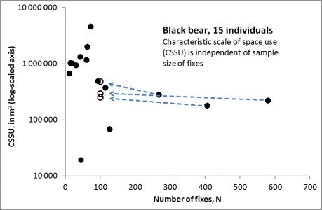
 However, consider the relationship between sample size, N, and the CSSU (right). F060 and F170 are found as the largest and smallest CSSU in the scatterplot. The average CSSU for all 15 individuals is ca 866,000 m2 (0.866 km2). Under constant conditions one should expect CSSU to be stationary under larger sample size (larger N) and non-autocorrelated series. However, the plot indicates a negative relationship between N and CSSU in these data, which is unexpected from the standard MRW model a priori (as shown by simulated data in this post)*.
Why? Many hypotheses may be invoked and tested – here I indicate one in particular. The capturing, radio collaring and subsequent tracking might have stressed the bears for some time after release. To study this, I re-analyzed the three individuals with the largest fix sampling period, including the first 100 fixes only. As shown by open symbols, all individuals (F182, F201 and F243) showed larger CSSU during the initial period for 100 fixes following release – a period of ca 1-2 years (!) – relative to the total fix sampling period of almost four years**, and thereby became similar to the other bears with respect to average spatial scale.
Is this an indication of a more restless space use behaviour in the first period following capture, release with radio collar and subsequent telemetry tracking 1-2 times/week (distance observer-animal is unknown)? To explore this aspect, several alternative hypotheses should also be considered (the three individuals were collared in August, June and June, and were 7, 3 and 3 years of age) – but the present pilot test does at least rise an interesting hypothesis. It also illustrates how the MRW model’s CSSU parameter may be applied to cast light on a potentially concerning aspect of data collection and its interpretation in the context of wildlife management***.
NOTES
*) In an upcoming post I will illustrate a transient effect in the early phase of home range establishment, and stationary CSSU for mature home range utilization. In the present context, is it reasonable to assume mature home ranges even for the initial 1-2 years of fix sampling.
**) Alternative methods to test for inter-sample difference in space use intensity abound, but have drawbacks. For example, the mean displacement length in a set of fix sampling intervals (lags) will be influenced by intermediate return events. Further, due to the very long-tailed (leptocurtic) distribution of step lengths in data from black bear, which has been verified to comply with the MRW space use model, comparing the relative difference in median displacement size in two or more samples is subject to large error terms due to the extreme outlier issue (“occasional sallies”). CSSU resolves these obstacles.
***) It should bee mentioned that the radio telemetry collars for black bear back in 1978 were substantially heavier than today’s standard. Triangulation also required close stalking to get a fix, in contrast to modern GPS.
REFERENCES
Gautestad, A. O., I. Mysterud, and M. R. Pelton. 1998. Complex movement and scale-free habitat use: testing the multi-scaled home range model on black bear telemetry data. Ursus 10:219-234.
Mandelbrot, B. B. 1983, The fractal geometry of nature. New York, W. H. Freeman and Company.
In the 1998 paper we applied the so-called re-scaled range analysis, R/SD (Mandelbrot 1983:pp247-25), to study home range area as a function of fix sample size. Details on the method and the raw data can be found in Gautestad et al. 1998. Below I revisit these bear data and re-test the Home range ghost function with the presently preferred method. Following this exercise I show a new result, which indicates that a collared bear’s characteristic scale of space use may have been inflated during the initial period of fix sampling of its path. Implicitly, the result rises the question if the experience of being collared and getting used to bearing the collar is influencing the bear’s space use towards a more coarse-grained habitat utilization on average; i.e., a larger CSSU, during the first months following the capture/release. The home range ghost regards the “paradoxical” pattern whereby home range area, A, apparently expands non-asymptotically with sample size of fixes, N, in compliance with the power law A = cNz. and z ≈ 0.5. The parameter c is the Characteristic scale of space use, CSSU, emerging from memory-dependent tendency to return to familiar locations.

The inset exemplifies the Home range ghost for one of the black bear individuals. The apparent area asymptote [inset, showing arithmetic axes for A(N)] disappears under log-transformation of the axes; i.e., the expansion with N is non-asymptotic and power law compliant with exponent z ≈ 0.5. Thus, the area expands with the square root of N.
In the present pilot test using a subset of 15 individual data sets (the first part of the total database of 77 series) the result shows strong coherence for estimates of z between the previous R/SD method and the present I(N) method with respect to how home range area responded to sample size, N. Once more I stress the advantage of using a model which accounts for the non-trivial N-dependency in home range size estimates, making CSSU – where the N-dependency is filtered out – a superior ecological proxy relative to the traditional method, direct area estimate.

As expected from scale-free space use, the distribution of CSSU is approximately log-normal (observe the log-scaling x-axis).
This histogram brings up interesting ecological questions. For example, why has the leftmost individual (female F170) 1:240 magnitude of CSSU – ca 1:15 in terms of linear rather than area scale – relative to the rightmost score (female F060)? In other words, according to the present analysis F170 utilized its habitat with substantially higher intensity than F060 (intensity ∝ 1/CSSU). F170 showed a relatively small I(N) for a given N, meaning that F170 utilized its habitat in a more area-restricted manner. Unfortunately I don’t have access to individual behaviour details nor environmental GIS data for the respective space use patterns.
Why? Many hypotheses may be invoked and tested – here I indicate one in particular. The capturing, radio collaring and subsequent tracking might have stressed the bears for some time after release. To study this, I re-analyzed the three individuals with the largest fix sampling period, including the first 100 fixes only. As shown by open symbols, all individuals (F182, F201 and F243) showed larger CSSU during the initial period for 100 fixes following release – a period of ca 1-2 years (!) – relative to the total fix sampling period of almost four years**, and thereby became similar to the other bears with respect to average spatial scale.
Is this an indication of a more restless space use behaviour in the first period following capture, release with radio collar and subsequent telemetry tracking 1-2 times/week (distance observer-animal is unknown)? To explore this aspect, several alternative hypotheses should also be considered (the three individuals were collared in August, June and June, and were 7, 3 and 3 years of age) – but the present pilot test does at least rise an interesting hypothesis. It also illustrates how the MRW model’s CSSU parameter may be applied to cast light on a potentially concerning aspect of data collection and its interpretation in the context of wildlife management***.
NOTES
*) In an upcoming post I will illustrate a transient effect in the early phase of home range establishment, and stationary CSSU for mature home range utilization. In the present context, is it reasonable to assume mature home ranges even for the initial 1-2 years of fix sampling.
**) Alternative methods to test for inter-sample difference in space use intensity abound, but have drawbacks. For example, the mean displacement length in a set of fix sampling intervals (lags) will be influenced by intermediate return events. Further, due to the very long-tailed (leptocurtic) distribution of step lengths in data from black bear, which has been verified to comply with the MRW space use model, comparing the relative difference in median displacement size in two or more samples is subject to large error terms due to the extreme outlier issue (“occasional sallies”). CSSU resolves these obstacles.
***) It should bee mentioned that the radio telemetry collars for black bear back in 1978 were substantially heavier than today’s standard. Triangulation also required close stalking to get a fix, in contrast to modern GPS.
REFERENCES
Gautestad, A. O., I. Mysterud, and M. R. Pelton. 1998. Complex movement and scale-free habitat use: testing the multi-scaled home range model on black bear telemetry data. Ursus 10:219-234.
Mandelbrot, B. B. 1983, The fractal geometry of nature. New York, W. H. Freeman and Company.