Statistical-mechanical Details on Space Use Intensity
While stronger intensity of space use in the standard (Markovian/mechanistic) biophysical model framework is equal to the proxy variable fix density, density=N/area, the complex system analogue is 1/c. This alternative expression for intensity is derived from from the Home range ghost formula I = cN0.5 = c√N). Below I illustrate the biophysical difference between the two intensity concepts by a simple Figure and some basic mathematics of the respective processes. The extended statistical mechanics of complex space use underscores the importance of estimating and applying a realistic spatial resolution, close to the magnitude of CSSU, when analyzing individual habitat utilization within various habitat classes. The traditional density variable for space use intensity will invoke a large noise term and even spurious results in ecological use/availability analyses of home range data.
In statistical-mechanical terms, one of the main discrepancies between the traditional space use models (mechanistic modelling) and complex movement (MRW) regards the representation of locally varying intensity of space use.
Classical space use intensity may be calculated from a single scale, and trivially extrapolated to a coarser resolution up to the full area extent.
 Why is this “freedom to zoom” feasible and mathematically allowed? Consider an example where the system extent is represented by the demarcation of a specific habitat type within a home range, simplified by a square under four conditions in the Figure to the right. Due to assumed compliance with standard statistical mechanics under classical space use analysis, we are specifically assuming finite system variance within the given spatial extent,
Var(X1) + Var(X2) + … + Var(Xn) = σ2
where [X] is the set of spatial elements from sectioning a system’s extent into sub-sets 1, 2 , 3 .., n; and sub-sets into sub-sub-sets to find respective sub-set variances. Thus, Var(Xi) is the i‘th element’s second moment variability (variance). For example, σ2 could be the intrinsic variances of the spatial inter-cell number of fixes in the virtual grid cells in the Figure above’s upper right scenario (sub-sub grid cells not shown).
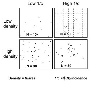
A spatial dispersion of a small and a large sample of fixes is shown in the upper and lower row, respectively. Two resolutions (spatial scales) are shown; the spatial extent (large squares) and a virtual grid scale (dotted lines, shown in the upper right square only). For interpretation of low and high intensity of complex space use, 1/c, see the main text.
The variance also changes proportionally with density. In other words, variance is stationary upon scaling and can thus be assumed to change proportionally with grid scale and density. This implies compliance with the central limit theorem. Even if intra-cell variance is not constant between grid cells at a given resolution within the given extent, as is expected in a heterogeneous habitat where local density varies, the sum of variance of these local parts is independent of this finer-scale variability between sub-components. Once again I underscore that this enormously simplifying system property regards scenaria under the standard statistical-mechanical framework!
On the other hand, the local variability of fix density from complex space use does not comply with the central limit theorem. Intensity of use needs to be calculated over a scale range – from “grain” to extent – rather than any scale, and the grain scale must be chosen with care.
Traditionally, space use may be quantified by the magnitude of “free space” (area/N) in a sample of N relocations (fixes) of an individual, due to compliance with the central limit theorem, as explained above. On the other hand we have complex space use; i.e., scale-free movement under influence of spatial memory and under compliance with the parallel processing postulate. Under this biophysical framework free space is expressed by the ratio area/√N, rather than the ratio area/N, and quantified by the characteristic scale of space use (CSSU). CSSU is a function of average movement speed and average return rate to previous locations. The system complexity from CSSU implies that the sum of the system parts’ standard deviation – rather than variance – is stationary upon re-scaling; i.e.,
s.d.(X1) + s.d.(X2) + … + s.d.(Xn) = √σ2
In other words, by default the spatial statistics follow a Cauchy distribution with scale parameter γ=1, rather than the classical Gaussian distribution. CSSU is proportional with the parameter c in the Home range ghost formula I=c√N, where I is number of fix-embedding virtual grid cells at spatial scale c≈CSSU.
What if we “lose focus” by studying the system (applying the grain scale) at coarser of finer resolutions than the CSSU? In the illustration above it is assumed that the superimposed virtual grid in the upper right corner reflects a spatial resolution that is close to this system’s true CSSU. If the system’s CSSU had been higher (1/c implicitly lower, as in the upper left-hand scenario), applying the same observer-defined grid resolution as in the upper right scenario would show deviance from the Cauchy distribution. The Cauchy scale parameter and the Home range ghost exponent are both inflated*) due to this “out of focus” situation; i.e., γ >> 1 and z >> 0.5
In short, by superimposing a virtual grid at scale much finer that CSSU, we will observe I ≈ cNz with z ≈ 1 rather than z ≈ 0.5. The parameter c and thus the true CSSU has been erratically estimated. The power exponent z → 1 as grid scale is successively decreased by using cells that are smaller than the true CSSU scale under this condition. However, compliance with z = 0.5 may be regained under a “Low 1/c” scenario (upper left) by sufficiently increasing the grid scale relative to cell sizes in the “large 1/c” scenario shown in the upper right example. We can then re-estimate CSSU by such scale zooming towards a coarser resolution and find that z → 0.5 as the coarse-graining is approaching the true CSSU. By comparing scenaria with low and high CSSU; i.e., high and low intensity of space use (1/CSSU), we can rise behavioural-ecological hypotheses about these differences. One obvious example regards strength of intra-home range habitat selection, but where intensity of space use is expressed by habitat-specific 1/c rather than density of fixes.
To summarize, while a “Gauss-compliant” (non-complex) kind of space use allows the average intensity of space use to be considered trivially constant upon zooming and linear rescaling over a scale range within the system extent, “Cauchy-compliant” space use requires a search for the correct grain scale to find the system’s average CSSU at this scale within the given extent.
More details on the statistical-mechanical system description of complex space use is found in my book.
NOTE
*) Apparently but erroneously, the variability under too fine-grained pixel resolution (grid cell scale) leading to z ≈ 1 and Cauchy scale parameter γ ≈ 2 may be interpreted as Gauss-compliant statistics. However, the Cauchy distribution does not have finite moments of any order. Thus, in strict terms, the reference to √σ2 under the γ = 1 scenario is not correct since variance is a term under standard statistical mechanics, but represents a commonly applied approximation (Mandelbrot 1983, Schroeder 1991).
REFERENCES
Mandelbrot, B. B. 1983, The fractal geometry of nature. New York, W. H. Freeman and Company.
Schroeder, M. 1991, Fractals, Chaos, Power Laws – Minutes from an Infinite Paradise. New York, W. H. Freedman and Company.
In statistical-mechanical terms, one of the main discrepancies between the traditional space use models (mechanistic modelling) and complex movement (MRW) regards the representation of locally varying intensity of space use.
Classical space use intensity may be calculated from a single scale, and trivially extrapolated to a coarser resolution up to the full area extent.
Var(X1) + Var(X2) + … + Var(Xn) = σ2
where [X] is the set of spatial elements from sectioning a system’s extent into sub-sets 1, 2 , 3 .., n; and sub-sets into sub-sub-sets to find respective sub-set variances. Thus, Var(Xi) is the i‘th element’s second moment variability (variance). For example, σ2 could be the intrinsic variances of the spatial inter-cell number of fixes in the virtual grid cells in the Figure above’s upper right scenario (sub-sub grid cells not shown).
A spatial dispersion of a small and a large sample of fixes is shown in the upper and lower row, respectively. Two resolutions (spatial scales) are shown; the spatial extent (large squares) and a virtual grid scale (dotted lines, shown in the upper right square only). For interpretation of low and high intensity of complex space use, 1/c, see the main text.
The variance also changes proportionally with density. In other words, variance is stationary upon scaling and can thus be assumed to change proportionally with grid scale and density. This implies compliance with the central limit theorem. Even if intra-cell variance is not constant between grid cells at a given resolution within the given extent, as is expected in a heterogeneous habitat where local density varies, the sum of variance of these local parts is independent of this finer-scale variability between sub-components. Once again I underscore that this enormously simplifying system property regards scenaria under the standard statistical-mechanical framework!
On the other hand, the local variability of fix density from complex space use does not comply with the central limit theorem. Intensity of use needs to be calculated over a scale range – from “grain” to extent – rather than any scale, and the grain scale must be chosen with care.
Traditionally, space use may be quantified by the magnitude of “free space” (area/N) in a sample of N relocations (fixes) of an individual, due to compliance with the central limit theorem, as explained above. On the other hand we have complex space use; i.e., scale-free movement under influence of spatial memory and under compliance with the parallel processing postulate. Under this biophysical framework free space is expressed by the ratio area/√N, rather than the ratio area/N, and quantified by the characteristic scale of space use (CSSU). CSSU is a function of average movement speed and average return rate to previous locations. The system complexity from CSSU implies that the sum of the system parts’ standard deviation – rather than variance – is stationary upon re-scaling; i.e.,
s.d.(X1) + s.d.(X2) + … + s.d.(Xn) = √σ2
In other words, by default the spatial statistics follow a Cauchy distribution with scale parameter γ=1, rather than the classical Gaussian distribution. CSSU is proportional with the parameter c in the Home range ghost formula I=c√N, where I is number of fix-embedding virtual grid cells at spatial scale c≈CSSU.
What if we “lose focus” by studying the system (applying the grain scale) at coarser of finer resolutions than the CSSU? In the illustration above it is assumed that the superimposed virtual grid in the upper right corner reflects a spatial resolution that is close to this system’s true CSSU. If the system’s CSSU had been higher (1/c implicitly lower, as in the upper left-hand scenario), applying the same observer-defined grid resolution as in the upper right scenario would show deviance from the Cauchy distribution. The Cauchy scale parameter and the Home range ghost exponent are both inflated*) due to this “out of focus” situation; i.e., γ >> 1 and z >> 0.5
In short, by superimposing a virtual grid at scale much finer that CSSU, we will observe I ≈ cNz with z ≈ 1 rather than z ≈ 0.5. The parameter c and thus the true CSSU has been erratically estimated. The power exponent z → 1 as grid scale is successively decreased by using cells that are smaller than the true CSSU scale under this condition. However, compliance with z = 0.5 may be regained under a “Low 1/c” scenario (upper left) by sufficiently increasing the grid scale relative to cell sizes in the “large 1/c” scenario shown in the upper right example. We can then re-estimate CSSU by such scale zooming towards a coarser resolution and find that z → 0.5 as the coarse-graining is approaching the true CSSU. By comparing scenaria with low and high CSSU; i.e., high and low intensity of space use (1/CSSU), we can rise behavioural-ecological hypotheses about these differences. One obvious example regards strength of intra-home range habitat selection, but where intensity of space use is expressed by habitat-specific 1/c rather than density of fixes.
To summarize, while a “Gauss-compliant” (non-complex) kind of space use allows the average intensity of space use to be considered trivially constant upon zooming and linear rescaling over a scale range within the system extent, “Cauchy-compliant” space use requires a search for the correct grain scale to find the system’s average CSSU at this scale within the given extent.
More details on the statistical-mechanical system description of complex space use is found in my book.
NOTE
*) Apparently but erroneously, the variability under too fine-grained pixel resolution (grid cell scale) leading to z ≈ 1 and Cauchy scale parameter γ ≈ 2 may be interpreted as Gauss-compliant statistics. However, the Cauchy distribution does not have finite moments of any order. Thus, in strict terms, the reference to √σ2 under the γ = 1 scenario is not correct since variance is a term under standard statistical mechanics, but represents a commonly applied approximation (Mandelbrot 1983, Schroeder 1991).
REFERENCES
Mandelbrot, B. B. 1983, The fractal geometry of nature. New York, W. H. Freeman and Company.
Schroeder, M. 1991, Fractals, Chaos, Power Laws – Minutes from an Infinite Paradise. New York, W. H. Freedman and Company.