Simulating Populations IIX: Time Series and Pink Noise
On rare occasions one’s research effort may lead to a Eureka! moment. While exploring and experimenting with the latest refinement of my Zoomer model for population dynamics I stumbled over a key condition to tune the model in and out of full coherence between spatial and temporal variability from the perspective of a self-similar statistical pattern. Fractal-like variability over space and time has been repeatedly reported in the ecological literature, but rarely has such pattern been studied simultaneously as two aspects of the same population. My hope is that the Zoomer model also has a more broadened potential by casting stronger light on the strange 1/f noise phenomenon (also called pink noise, or Flicker noise), which still tends to create paradoxes between empirical patterns and theoretical models in many fields of science.
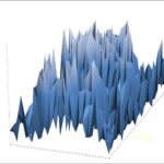 First, consider again some basic statistical aspects of a Zoomer-based simulation. Above I show the spatial dispersion of individuals within the given arena. See previous posts I-VII in this series for other examples, system conditions and technical details. The new aspect in the present post is a toggle towards temporal variation of the spatial dispersion, and fractal properties in that respect (called a self-affine pattern in a series of measurements, consistent with 1/f noise*. This phenomenon usually indicates the presence of a broad distribution of time scales in the system.
 In particular, observe the log(M,V) regression. As in previous examples, the variable M in the Taylor’s power law model V = aMb represents – in my application of the law – a combination of the average number of individuals in a set of samples at different locations at a given scale and supplemented by samples of M at different scales. The latter normally contributes the most to the linearity of the log(M,V) plot, due to a better spread-out of the range of M.
 During the present scenario that was run for 5000 time steps after skipping an initial transient period, the self-similar and self-organized spatial pattern of slope b ≈ 2 and log(a) ≈ 0 was dominating, only occasionally interrupted by some short intervals with b << 2 and log(a) >> 0. These episodes were caused by simultaneous disruption of a relatively high number of local populations in cells that exceeded their respective carrying capacity level (CC), leading to a lot of simultaneous re-positioning of these individuals to other parts of the arena in accordance to the actual simulation rules. Thus, some temporary “disruptive noise” could appear now and then, occasionally leading to a relatively scrambled population dispersion with b ≈ 1 (Poisson distribution) and log(a) >> 0 for short periods of time.

The actual time series for the present example is given above, showing local density at a given location (a cell at unit scale) over a period of 5,000 increments. The scramble events due to many simultaneous population crashes in other cells over the arena can indirectly be seen as the strongest density peaks in the series. The sudden inflow of immigrants to the given locality caused a disruption to the monitored local population, which typically crashed during the next increment due to density > CC.
In may respects the series illustrates the “frustrating” phenomenon seen in long time series in ecology: the longer the observation period, the larger the accumulated magnitude of fluctuations (Pimm and Redfearn 1988, Pimm 1991). However, in the present scenario where conditions are known, there is no uncertainty related to whether the complex fluctuations are caused by extrinsic (environmental) or intrinsic dynamics. Since CC was set to be uniform over space and time and only varied due to some level of stochastic noise (a constant + a smaller random number) the time series above is expressing intrinsically driven, self-organized kind of fluctuations over space, time and scale.
The key lesson from the present analysis is to understand local variability as a function not only of local conditions, but also a function of coarser-scale events and conditions in the surroundings of the actual population being monitored. The latter is often referred to a long-range dependence. In the Zoomer model this phenomenon is rooted in the emergence of scale-free space use of the population, due to scale-free space use at the individual level (the Multi-scaled random walk model). In the present post I illustrate long-range dependence also over temporal variability.
 To remove the major magnitude of serial autocorrelation the original series above was sampled 1:80. The correlogram to the right shows this frequency to be a feasible compromise between full non-autocorrelation and a reasonably long remaining series length.
 After this transformation towards observing the series at a different scale, the sampled series was subject to log(Mt,V) analysis, where Mt represents – in a sliding window manner – the mean abundance over a few time steps of the temporally coarser-scaled series, and V represents these intervals’ respective variance.
Interestingly, the log(Mt,V) pattern was reasonably similar to the log(M,V) pattern from the spatial transect above; i.e., the marked line with b ≈ 2 and log(a) ≈ 0, under the condition that the series was analyzed at a sufficiently coarse temporal scale from sampling to avoid most of the serial autocorrelation.
The most intriguing result is perhaps the Figure below, showing the log-log transformed power spectrogram of the original time series**. Over a temporal scale range up to frequency of 1500 (the x-axis) the distribution of power (the y-axis); i.e., amplitudes squared, satisfies 1/f noise!
 See my book for an introduction to this statistical “beast” ***, where I devote several chapters to it. At higher frequencies further down towards the “rock bottom” of 4096 (the dimmed area), the power shows inflation. This is probably due to an integer effect at the finest resolutions of the time series, since individuals always come as whole numbers rather than fractions. Thus, the finest-resolved peak in power was probably influenced by this effect.
To my knowledge, no other model framework has simultaneously been able to reproduce the empirically often reported fractal-like spatial population abundance (the spatial expression of Taylor’s power law) with a fractal-like temporal variation (the temporal Taylor’s power law). Only either-or results have been previously reproduced by models among the thousands of papers on this topic over the last 60 years or so.
For an introduction to 1/f noise in an ecological context, you may find this link to a review by Halley and Inchausti (2004) helpfull. I cite:
1/f-noises share with ecological time series a number of important properties: features on many scales (fractality), variance growth and long-term memory. (…) A key feature of 1/f-noises is their long memory. (…) Given the undoubted ubiquity and importance of 1/f-noise, it is surprising that so much work still revolves about either observing the 1/f-noise in (yet more) novel situations, or chasing what seems to have become something of a “holy grail” in physics: a universal mechanism for 1/f-noise. Meanwhile, important statistical questions remain poorly understood.
What about ecological methods based on the theory above? By exploring the statistical pattern of animal dispersion over space and its variability over time – and mimicking this pattern in the Zoomer model – a wide range of ecological aspects may be studied within a hopefully more realistic framework than the presently dominating approach using coupled map lattice models or differential equations. Statistical signatures of quite novel kind can be extracted from real data and interpreted in the light of complex space use theory.
In upcoming posts I will on one hand dig into the set of Zoomer model “knobs” that steer the statistical pattern in and out of – for example – the 1/f noise condition, and on the other hand I will exemplify the potential for ecological applications of the model.
NOTES
*) “1/f-noise” refers to 1/fν-noise for which 0 ≤ ν ≤ 2; “near-pink 1/f-noise” refers to cases where 0.5 ≤ ν ≤ 1.5 and “pink noise” refers to the specific case were ν = 1. All 1/fν-noises are defined by the shape of their power spectrum S(ω):
S ∝ 1/ων
Here ω = 2πf is the angular frequency. “White noise” is characterized by ν ≈ 0, and its integral, “red” or “brown” noise, has ν ≈ 2. A classical random walk along a time axis is an example of the latter, and its derivative produces white noise.
**) Since a FFT analysis requires a series length satisfying a power or 2, only the first 4096 steps were included.
***) 1/f noise is challenging, both mathematically and conceptually:
The non-integrability in the cases ν ≥ 1 is associated with infinite power in low frequency events; this is called the infrared catastrophe. Conversely for ν ≤ 1, which contains infinite power at high frequencies, it is called the ultraviolet catastrophe. Pink noise (ν = 1) is non-integrable at both ends of the spectrum. The upper and lower frequencies of observation are limited by the length of the time series and the resolution of the measurement, respectively.
Halley and Inchausti (2004), p R7.
REFERENCES
Halley, J. M. and P. Inchausti. 2004. The increasing importance of 1/f noises as models of ecological variability. Fluctuation and Noise Letters 4:R1–R26.
Pimm, S. L. 1991, The balance of nature? Ecological issues in the conservation of species and communities. Chicago, The University of Chicago Press.
Pimm, S. L., and A. Redfearn. 1988. The variability of animal populations. Nature 334:613-614.

The actual time series for the present example is given above, showing local density at a given location (a cell at unit scale) over a period of 5,000 increments. The scramble events due to many simultaneous population crashes in other cells over the arena can indirectly be seen as the strongest density peaks in the series. The sudden inflow of immigrants to the given locality caused a disruption to the monitored local population, which typically crashed during the next increment due to density > CC.
In may respects the series illustrates the “frustrating” phenomenon seen in long time series in ecology: the longer the observation period, the larger the accumulated magnitude of fluctuations (Pimm and Redfearn 1988, Pimm 1991). However, in the present scenario where conditions are known, there is no uncertainty related to whether the complex fluctuations are caused by extrinsic (environmental) or intrinsic dynamics. Since CC was set to be uniform over space and time and only varied due to some level of stochastic noise (a constant + a smaller random number) the time series above is expressing intrinsically driven, self-organized kind of fluctuations over space, time and scale.
The key lesson from the present analysis is to understand local variability as a function not only of local conditions, but also a function of coarser-scale events and conditions in the surroundings of the actual population being monitored. The latter is often referred to a long-range dependence. In the Zoomer model this phenomenon is rooted in the emergence of scale-free space use of the population, due to scale-free space use at the individual level (the Multi-scaled random walk model). In the present post I illustrate long-range dependence also over temporal variability.

Interestingly, the log(Mt,V) pattern was reasonably similar to the log(M,V) pattern from the spatial transect above; i.e., the marked line with b ≈ 2 and log(a) ≈ 0, under the condition that the series was analyzed at a sufficiently coarse temporal scale from sampling to avoid most of the serial autocorrelation.
The most intriguing result is perhaps the Figure below, showing the log-log transformed power spectrogram of the original time series**. Over a temporal scale range up to frequency of 1500 (the x-axis) the distribution of power (the y-axis); i.e., amplitudes squared, satisfies 1/f noise!

To my knowledge, no other model framework has simultaneously been able to reproduce the empirically often reported fractal-like spatial population abundance (the spatial expression of Taylor’s power law) with a fractal-like temporal variation (the temporal Taylor’s power law). Only either-or results have been previously reproduced by models among the thousands of papers on this topic over the last 60 years or so.
For an introduction to 1/f noise in an ecological context, you may find this link to a review by Halley and Inchausti (2004) helpfull. I cite:
1/f-noises share with ecological time series a number of important properties: features on many scales (fractality), variance growth and long-term memory. (…) A key feature of 1/f-noises is their long memory. (…) Given the undoubted ubiquity and importance of 1/f-noise, it is surprising that so much work still revolves about either observing the 1/f-noise in (yet more) novel situations, or chasing what seems to have become something of a “holy grail” in physics: a universal mechanism for 1/f-noise. Meanwhile, important statistical questions remain poorly understood.
What about ecological methods based on the theory above? By exploring the statistical pattern of animal dispersion over space and its variability over time – and mimicking this pattern in the Zoomer model – a wide range of ecological aspects may be studied within a hopefully more realistic framework than the presently dominating approach using coupled map lattice models or differential equations. Statistical signatures of quite novel kind can be extracted from real data and interpreted in the light of complex space use theory.
In upcoming posts I will on one hand dig into the set of Zoomer model “knobs” that steer the statistical pattern in and out of – for example – the 1/f noise condition, and on the other hand I will exemplify the potential for ecological applications of the model.
NOTES
*) “1/f-noise” refers to 1/fν-noise for which 0 ≤ ν ≤ 2; “near-pink 1/f-noise” refers to cases where 0.5 ≤ ν ≤ 1.5 and “pink noise” refers to the specific case were ν = 1. All 1/fν-noises are defined by the shape of their power spectrum S(ω):
S ∝ 1/ων
Here ω = 2πf is the angular frequency. “White noise” is characterized by ν ≈ 0, and its integral, “red” or “brown” noise, has ν ≈ 2. A classical random walk along a time axis is an example of the latter, and its derivative produces white noise.
**) Since a FFT analysis requires a series length satisfying a power or 2, only the first 4096 steps were included.
***) 1/f noise is challenging, both mathematically and conceptually:
The non-integrability in the cases ν ≥ 1 is associated with infinite power in low frequency events; this is called the infrared catastrophe. Conversely for ν ≤ 1, which contains infinite power at high frequencies, it is called the ultraviolet catastrophe. Pink noise (ν = 1) is non-integrable at both ends of the spectrum. The upper and lower frequencies of observation are limited by the length of the time series and the resolution of the measurement, respectively.
Halley and Inchausti (2004), p R7.
REFERENCES
Halley, J. M. and P. Inchausti. 2004. The increasing importance of 1/f noises as models of ecological variability. Fluctuation and Noise Letters 4:R1–R26.
Pimm, S. L. 1991, The balance of nature? Ecological issues in the conservation of species and communities. Chicago, The University of Chicago Press.
Pimm, S. L., and A. Redfearn. 1988. The variability of animal populations. Nature 334:613-614.