Simulating Populations V: Bottlenecks and Recovery
Time to simulate a stress-test of the two population-kinetic frameworks, the traditional Coupled map lattice model and the novel Zoomer model! Consider a scenario where some kind of environmental event has crushed the population to about 1% of its normal carrying capacity. In addition, the remaining population has also become spatially fragmented during this catastrophe. Then consider that the condition improves to the pre-crash level. What is the population’s potential to recover under the two scenaria you have become familiar with in Parts I-IV, scale-specific and scale-free kinetics?
 The map to the right shows the small population’s spatial dispersion at the start of the potential recovery phase. Isopleths indicate local population density, which shows an average of 165 individuals pr. occupied cell at unit scale while the carrying capacity (CC) has been restored to a potential for 5,000 individuals at this scale. In other words, in this scenario most local populations have gone extinct as a consequence of the recent crunch event.
 Then the recovery phase begins. Starting with the standard condition of scale-specific population dynamics/kinetics (Coupled map lattice model) and setting diffusion rate at unit scale to 5% between cells and net population growth of 2%, the following image to the left the population dispersion after 20 iterations.
Since the diffusion rate is larger than the local growth rate (the general condition of spatially unconstrained animal populations, since reproduction is a relatively slow process compared to movement) and the population is now surrounded by unoccupied area, the population is drifting towards extinction!
 This fate is also facilitated by an additional model condition, Allée effects. At this low level of population abundance it is important to consider and implement three aspects: First, accelerated extinction at very low abundance levels have to be introduced. Here I set the critical level to 50 individuals pr. unit cell*. Below this level, the population is reduced by 10% pr. time increment. Second, due to the low abundance levels, one has to consider that individuals exist as discrete entities, not fractions of numbers (at high abundance the difference between discrete and continuous numbers are insignificant). Third, at very low population densities random events take its toll. I implement this as some noise level on the survival rate in the Allée zone; i.e., in cells with less than 50 individuals.
 In contrast, under otherwise identical conditions does scale-free and memory-influenced zooming influence the population’s otherwise dire fate after the catastrophic event? Obviously it does.

Since the diffusion rate is larger than the local growth rate (the general condition of spatially unconstrained animal populations, since reproduction is a relatively slow process compared to movement) and the population is now surrounded by unoccupied area, the population is drifting towards extinction!
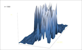
The Zoomer snapshots below at t=20, t= 200, t= 500 and t= 1,000 shows a population in healthy recovery, despite being surrounded by a wide zone of unoccupied space. The 5% diffusion rate under the CML condition above is replaced by a 5% zooming rate (“exploratory steps”, as seen from the individual perspective), with 1% conspecific attraction kind of redistribution pr. scale level (see previous parts of this series). In other respects the conditions are similar to the CML model, including net growth being smaller than individual reshuffling at unit scale.
 Below, the log(M,V) result at t = 1,000 (as in the earlier parts of recovery; not shown) shows full compliance with intercept ≈ 0 and slope ≈ 2, as predicted by the Zoomer model.
Due to a CLM's intrinsic design of Markovian, scale-specific dynamics, it ultimately - in an open environment - makes a population susceptible to extinction. On the other hand, memory-influenced and scale-free dynamics allows for population-saving intraspecific cohesion under similar environmental conditions and events. In this manner the Zoomer model illustrates – and potentially resolves – some crucial but under-communicated issues with respect to the standard modelling framework.
 Inclusion of spatial memory and strategic space use – in particular the capacity for individuals to include conspecifics as part of their resource map at strategic scales (conspecific attraction) – counteracts the otherwise detrimental effect of living in an open world. At the fringe of any animal population, under the standard modelling paradigm local abundance is constantly threatened by individuals getting lost in space, by drifting away from sufficiently strong contact with conspecifics (ref: diffusion and Allée effects).
 The Zoomer design, by implementing spatio-temporal memory, formulates a solution to this core problem for population dynamical modelling. However, the solution requires an extended kind of statistical mechanics. Read my book – for the time being the main source (and for some parts the only source) for a theoretical overview of this approach!
In the next post I will address an expected primary objection to my quite far-fetching conclusions above, that traditional population dynamical modelling is based on shaky assumptions with respect to realism. In future posts I will also present empirical support for the Zoomer model.
NOTE
*) There is nothing magic about N=50, but to avoid a more complicated formula for the Allée effect – with little or no advantage with respect to model realism in over-all terms – I have just chosen a “small abundance number” relative to the carrying capacity.
Due to a CLM's intrinsic design of Markovian, scale-specific dynamics, it ultimately - in an open environment - makes a population susceptible to extinction. On the other hand, memory-influenced and scale-free dynamics allows for population-saving intraspecific cohesion under similar environmental conditions and events. In this manner the Zoomer model illustrates – and potentially resolves – some crucial but under-communicated issues with respect to the standard modelling framework.


In the next post I will address an expected primary objection to my quite far-fetching conclusions above, that traditional population dynamical modelling is based on shaky assumptions with respect to realism. In future posts I will also present empirical support for the Zoomer model.
NOTE
*) There is nothing magic about N=50, but to avoid a more complicated formula for the Allée effect – with little or no advantage with respect to model realism in over-all terms – I have just chosen a “small abundance number” relative to the carrying capacity.