Simulating Populations IX: Tuning a Classic CML Model In and Out of Pink Noise

In the previous post I presented a time series of the Zoomer model, verifying a 1/f (pink) noise signature. For the sake of comparison I here present a series from scale-specific dynamics (standard Coupled map lattice model) using a comparable system setup. Interestingly, some specific similarities with some statistical aspects of the Zoomer model is appearing, given some “Fine tuning” of conditions. However, some aspects are able to pinpoint the difference anyway.

The present CML model conditions are the same as for the Zoomer version with 5-scale zooming of 1% zoomers pr. scale level and time increment, except for replacing zooming with 1% diffusion between neighbour cells at unit scale. Recall from previous posts in this series – and from the older post where the Zoomer model was described in mathematical terms (search Archive) – that zooming has a component of intraspecific cohesion. In contrast, diffusion is a memory-less (Markov compliant) kind of re-distribution of individuals.

The spatial density snapshot (upper left) shows the smooth surface expected from even a weak magnitude of memory-less inter-cell mixing. Also observe the intercept log(a) << 0 in the log(M,V) plot.

By the way, such a smooth surface is what modelers of population dynamics tend to love, since it adheres to the mean field property. On the other hand, empirical data typically shows a very rugged surface over a wide range of resolutions (even in a relatively homogeneous environment), statistically in close compliance with what the Zoomer model generates.

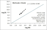
At this particular instance in time of the CML simulation above one also sees the effect from a local cell overshooting its carrying capacity (CC) and redistributing its individuals as small swarms among some of the other cells (seen as temporary “warts” on the density surface). The log(M,V) plot shows a slope close to b = 2 and log(a) << 0, as in previous examples of scale-specific CML dynamics. I have previously pointed out that log(a) << 0 (in combination with b ≈ 2) is a hallmark of scale-specific rather than scale-free population dispersion. It does not comply with the “CV = 1” law for scale-free dynamics [b ≈ 2, log(a) ≈ 0]. Now and then some larger number of simultaneous local population breakdown happen, and – as was shown also for the Zoomer condition – this led to a temporary change to b≈1 and log(a) >> 0.

The actual time series (above) appears qualitatively different from the Zoomer equivalent (see Part IIX), being less rugged. Despite this, the correlogram above from a sampled series at frequency 1:80 does not reveal any significant difference to the Zoomer model result. However, the log(M_t,V) plot is both more clustered and with a generally smaller magnitude of log(V) than was found in the Zoomer example.

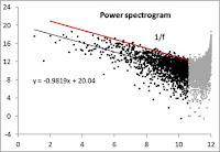
Surprisingly, the power spectrogram (log₂-transformed) to the left satisfies pink noise; 1/f^μ with μ ≈ 1), and is thus similar to the zoomer example in the previous post.

However, as shown to the right if local population survival when density overshoots CC is increased from 0% to 60%, the spectrum is more flattened (more like white noise). In comparison, a similar change to the CC overshoot behaviour for the Zoomer model did not change the spectrum away from 1/f (below, right).

What regards the other statistical aspects of the present zoomer example with CC survival 60%, these are also reproduced below.

Despite a more “noisy” time series than the 0% local survival condition (see image below for 60%, and compare with Part IIX for 0%), which is also reflected in spatial log(M,V) with b ≈ 1.5 and log(a) >> 0 dominating most of the time (during more silent intervals the CV=1 law applies), the temporal log(M,V) plot below shows larger log(V) for a given log(M), relative to the CML example. Thus, despite the narrow range of log(M) the level of log(V) the zoomer example with survival rate 60% is at least close to the line for b ≈ 2.

In summary, by setting CC overshoot survival low the traditional population dynamical modelling approach to apply scale-specific coupled map lattice models may to some degree mimic scale-free pattern generation with respect to the power spectrum (in this instance, survival = 0%, where “survival” implies remaining individuals in the given cell while most of the emigrants survive but redistribute themselves to other cells). On the other hand, the Zoomer model shows stronger statistical resilience over a broader range of conditions, including both the power spectrum and the CV ≈ 1 property.

In a follow-up post I will reveal further theoretical details, by linking the Zoomer model to so-called self-organized criticality in statistical mechanics of complex systems. Step-by-step I am approaching a shift towards ecological application of the Zoomer model. However; by necessity, theory first.