Simulating Populations X: Confronting Theory With Real Data
In Part IX a standard Coupled map lattice model was shown to be able to display a 1/f power spectrum, by careful tuning of one of the conditions for population mixing. On the other hand, I also showed that the Zoomer model under similar general conditions showed a higher resilience with respect to the 1/f property. In the present post I explore this statistical resilience of the Zoomer model further, by stressing the population system towards other corners of extreme conditions. However, I start by elaborating on this pressing question: Why this recurrent focus on 1/f noise? To stimulate your curiosity I also reproduce from my book two analyses of empirical data; the sycamore aphid Drepanosiphum platanoides and the leaf miner Leucoptera meyricki.
First, a brief bird’s view of complex dynamics. I have repeatedly given partly answers to the question “why focusing on 1/f noise?”, but here I seek to give you a broader perspective, starting with a citation from Scholarpedia:
1/f fluctuations are widely found in nature. During 80 years since the first observation by Johnson (1925), long-memory processes with long-term correlations and 1/fα (with 0.5 ≲ α ≲ 1.5) behavior of power spectra at low frequencies f have been observed in physics, technology, biology, astrophysics, geophysics, economics, psychology, language and even music… …1/f noise can not be obtained by the simple procedure of integration or of differentiation of such convenient signals. Moreover, there are no simple, even linear stochastic differential equations generating signals with 1/f noise. The widespread occurrence of signals exhibiting such behavior suggests that a generic mathematical explanation might exist. Except for some formal mathematical descriptions like fractional Brownian motion (half-integral of a white noise signal), however, no generally recognized physical explanation of 1/f noise has been proposed. Consequently, the ubiquity of 1/f noise is one of the oldest puzzles of contemporary physics and science in general.
Ward and Greenwood (2007)
As scientists – whether we are ecologists or working in other fields – we are of course curious about exploring this hard nut to crack, in particular since natural populations (paradoxically, if judged by expectation from standard theory) tend to show 1/f noise in their spatial variation and temporal fluctuations. Here are two examples from my book:
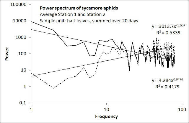

Both series show close agreement with 1/f noise; and their respective derivatives trivially show similar compliance with 1/f noise (power changing proportionally with frequency, shown as dashed plots). The first example is a spatial transect of sycamore aphids (my own data), and the second example shows my power spectrogram analysis based on a time series collected from Bigger and Tapley (1969) of the coffee leaf miner Leucoptera meyricki. Both data sets and methods are described in detail in my book.
The burning question then arises: what kind of spatially extended population model may reproduce 1/f noise over space, time and scale? Within the current paradigm the coupled map lattice (CML) approach fails, since it by design cannot reproduce long distance and far back influence on a present location’s dynamics*.The standard calculus approach (ordinary and partial differential equations) also fails, since models of this design rests on the mean field approximation. In short a novel approach is needed.
As previously stated, for the time being and to my knowledge the Zoomer model is the only candidate standing the test when confronting simulations with real data properties with respect to statistical mechanics.
In a series of posts I have now in a step-by step manner presented the Zoomer model, and compared it with the paradigmatic approach in the field, the coupled map lattice design (CML). In Part IX the CML model was shown to be more sensitive to the population’s response to local overcrowding (the CC level). Only 100% redistribution of individuals where CC was temporally exceeded led to a 1/f pattern. The Zoomer model showed 1/f, whether 40% or 100% of individuals emigrated. In other words, strong statistical resilience in this regard. However, the best way to test a model’s intrinsic dynamics is to stress it to its limit. Thus, below I test the effect from changing the redistribution behaviour of the individuals that emigrate from the “CC overshoot” localities.
So far, these individuals have been set to redistribute themselves to other cells in “swarms” of X% each of all swarmers at the actual point in time. For example, if two cells have an overshoot event at this point in time with a total number of dispersers of – say – 10,000 individuals, these dispersers settle in 5% of the other cells (of 1024 cells available) in swarms of ≈ 195 individuals pr. receiving cell, chosen randomly.
 Below I explore two variants of this behaviour; (1) the dispersers settle randomly and individually among the available cells, and (2) the dispersers settle in only 1% of the cells. The former implies a more smooth dispersal kernel, and the latter a more collective kind of large swarms settling in just a few cells.
 In short, the power spectrum of the time series of the smooth dispersal condition shows white noise (1/f0), while the extremely clumped dispersal shows more like red noise (1/f1.8).**
 To conclude, the 1/f property in the Zoomer model seems to be critically sensitive to the behaviour of the dispersing individuals during local crowding (boom/bust) events. Whether the bust leads to local meltdown (0% remaining) or not (60% remaining), the 1/f pattern was robust. However, how the emigrating individual re-settled themselves (independently or in a contagious manner) determined 1/f compliance. An intermediate level of contagion was in best compliance with 1/f, and thereby with the empirical results shown above. Intermediate contagion implies intermediate level of population disturbance frequency***.
 This conclusion also fits well with the general model property of zooming, which reflects conspecific attraction in over-all terms. The “balanced” and intermediate kind of zooming follows prom the generic condition that the strength of zooming is distributed evenly over that actual range of spatial scales (k–b zoomers to kb larger grid area, with b=1). However, while zoomers re-distribute themselves contagiously in a spatially explicit manner from a process that depends on the individuals’ spatial memory of past experiences, the swarms of emigrants in the current Zoomer design settle randomly. “Stressed” individuals (emigrants from local crunch events) are assumed to redistribute themselves in a tactical manner, temporarily following the collective behaviour of a swarm during the actual time increment.
 Interestingly, the spatial pattern log(M,V) for the white noise condition shows – as expected – a similarly rattled pattern, with slope b ≈ 1 and log(a) >> 0. However, in the contageous dispersal scenario, the spatially self-similar property b ≈ 2 and log(a) ≈ 0 is maintained. Hence, the spatial pattern is still fractal-compliant with similar properties as for other levels of contagion during re-distribution events, despite the more classic “random walk-like” time series of fluctuations.
 To conclude, by studying a population’s variation of abundance over space, time and scale it should be possible to analyze a wide range of key ecological signatures from the data series’ statistical properties; for example to what extent the population under the given environmental conditions adheres to a multi-scaled and scale-free kind of intrinsically driven population dynamics/kinetics, and how the population responds to local crowding events.
Hopefully, this statistical-mechanical approach may lead to more realistic theory and thus better predictive power. Bringing population dynamical modelling and some basic empirical properties of real populations in closer agreement is long overdue in this important field of ecology.
Crucially, these basic analyses should also be able to cast light on to what extent the dynamics are compliant with expectations from a classical modeling regime; i.e., a Markov- and mean field compliant kind of statistical mechanics, or the alternative framework based on the parallel processing conjecture for individual space use (the MRW model and its population level version, the Zoomer model). This challenge is of course the first obstacle that has to be passed. Hopefully the two insect examples above will inspire others to perform broader and deeper tests – for example, based on my recent series of blog posts.
NOTES
*) The 1/f pattern from a CML example in Part IX was a 1/f look-alike due to some tweaking of conditions, but it failed when other statistical aspects were scrutinized.
**) As in previous scenaria, the time scale is set to be smaller than the population’s net growth rate of 0-1%, giving a focus of the higher rate population mixing processes; diffusion 1% for the CML examples, zooming 5% in the Zoomer examples (distributed with 1% pr. spatial scale), and a stochastic magnitude of intrinsic re-distribution of individuals from local CC-linked events under both platforms.
***) By intermediate frequency of disturbance from intrinsic reshuffling of individuals I mean on one side that a given locality’s frequency of disruptions by swarms of dispersing individuals from other localities depends on swarm size. Larger swarms mean fewer locations where they settle. On one hand, large swarms (stronger contagion among emigrants) appear more rarely at a given locality in statistical terms but will have stronger local impact when a swarm arrives. On the other hand, an additional disruptive event from such an influx may happen within the next time increment if the sum of existing and arriving individuals surpass the local CC level. One also has to consider that a higher local abundance due to arriving immigrants may change a declining local abundance to an increasing one due to the zooming process of conspecific attraction.The abundance level as seen from a broader neighbourhood scale may increase sufficiently to toggle this neighbourhood (including the actual cell receiving the immigrants) from being a net supplier; i.e., subject to net local population decline, to becoming net receiver of individuals in the time ahead.
This perspective again underscores the importance of studying population dynamics not only over space and time, but also over respective scale axes and in a Parallel processing manner. Hence, a Markovian-compliant model framework is not sufficient to understand complex dynamics/kinetics, including the 1/f property.
REFERENCES
Bigger, M., and R. G. Tapley. 1969. Prediction of outbreaks of coffee leaf-miners on Kilimanjaro. Bulletin of Entomological Research 58:601-618.
Ward, L. M. and P. E. Greenwood. 2007. 1/f noise. Scholarpedia 2(12):1537.
First, a brief bird’s view of complex dynamics. I have repeatedly given partly answers to the question “why focusing on 1/f noise?”, but here I seek to give you a broader perspective, starting with a citation from Scholarpedia:
1/f fluctuations are widely found in nature. During 80 years since the first observation by Johnson (1925), long-memory processes with long-term correlations and 1/fα (with 0.5 ≲ α ≲ 1.5) behavior of power spectra at low frequencies f have been observed in physics, technology, biology, astrophysics, geophysics, economics, psychology, language and even music… …1/f noise can not be obtained by the simple procedure of integration or of differentiation of such convenient signals. Moreover, there are no simple, even linear stochastic differential equations generating signals with 1/f noise. The widespread occurrence of signals exhibiting such behavior suggests that a generic mathematical explanation might exist. Except for some formal mathematical descriptions like fractional Brownian motion (half-integral of a white noise signal), however, no generally recognized physical explanation of 1/f noise has been proposed. Consequently, the ubiquity of 1/f noise is one of the oldest puzzles of contemporary physics and science in general.
Ward and Greenwood (2007)
As scientists – whether we are ecologists or working in other fields – we are of course curious about exploring this hard nut to crack, in particular since natural populations (paradoxically, if judged by expectation from standard theory) tend to show 1/f noise in their spatial variation and temporal fluctuations. Here are two examples from my book:


Both series show close agreement with 1/f noise; and their respective derivatives trivially show similar compliance with 1/f noise (power changing proportionally with frequency, shown as dashed plots). The first example is a spatial transect of sycamore aphids (my own data), and the second example shows my power spectrogram analysis based on a time series collected from Bigger and Tapley (1969) of the coffee leaf miner Leucoptera meyricki. Both data sets and methods are described in detail in my book.
The burning question then arises: what kind of spatially extended population model may reproduce 1/f noise over space, time and scale? Within the current paradigm the coupled map lattice (CML) approach fails, since it by design cannot reproduce long distance and far back influence on a present location’s dynamics*.The standard calculus approach (ordinary and partial differential equations) also fails, since models of this design rests on the mean field approximation. In short a novel approach is needed.
As previously stated, for the time being and to my knowledge the Zoomer model is the only candidate standing the test when confronting simulations with real data properties with respect to statistical mechanics.
In a series of posts I have now in a step-by step manner presented the Zoomer model, and compared it with the paradigmatic approach in the field, the coupled map lattice design (CML). In Part IX the CML model was shown to be more sensitive to the population’s response to local overcrowding (the CC level). Only 100% redistribution of individuals where CC was temporally exceeded led to a 1/f pattern. The Zoomer model showed 1/f, whether 40% or 100% of individuals emigrated. In other words, strong statistical resilience in this regard. However, the best way to test a model’s intrinsic dynamics is to stress it to its limit. Thus, below I test the effect from changing the redistribution behaviour of the individuals that emigrate from the “CC overshoot” localities.
So far, these individuals have been set to redistribute themselves to other cells in “swarms” of X% each of all swarmers at the actual point in time. For example, if two cells have an overshoot event at this point in time with a total number of dispersers of – say – 10,000 individuals, these dispersers settle in 5% of the other cells (of 1024 cells available) in swarms of ≈ 195 individuals pr. receiving cell, chosen randomly.


Hopefully, this statistical-mechanical approach may lead to more realistic theory and thus better predictive power. Bringing population dynamical modelling and some basic empirical properties of real populations in closer agreement is long overdue in this important field of ecology.
Crucially, these basic analyses should also be able to cast light on to what extent the dynamics are compliant with expectations from a classical modeling regime; i.e., a Markov- and mean field compliant kind of statistical mechanics, or the alternative framework based on the parallel processing conjecture for individual space use (the MRW model and its population level version, the Zoomer model). This challenge is of course the first obstacle that has to be passed. Hopefully the two insect examples above will inspire others to perform broader and deeper tests – for example, based on my recent series of blog posts.
NOTES
*) The 1/f pattern from a CML example in Part IX was a 1/f look-alike due to some tweaking of conditions, but it failed when other statistical aspects were scrutinized.
**) As in previous scenaria, the time scale is set to be smaller than the population’s net growth rate of 0-1%, giving a focus of the higher rate population mixing processes; diffusion 1% for the CML examples, zooming 5% in the Zoomer examples (distributed with 1% pr. spatial scale), and a stochastic magnitude of intrinsic re-distribution of individuals from local CC-linked events under both platforms.
***) By intermediate frequency of disturbance from intrinsic reshuffling of individuals I mean on one side that a given locality’s frequency of disruptions by swarms of dispersing individuals from other localities depends on swarm size. Larger swarms mean fewer locations where they settle. On one hand, large swarms (stronger contagion among emigrants) appear more rarely at a given locality in statistical terms but will have stronger local impact when a swarm arrives. On the other hand, an additional disruptive event from such an influx may happen within the next time increment if the sum of existing and arriving individuals surpass the local CC level. One also has to consider that a higher local abundance due to arriving immigrants may change a declining local abundance to an increasing one due to the zooming process of conspecific attraction.The abundance level as seen from a broader neighbourhood scale may increase sufficiently to toggle this neighbourhood (including the actual cell receiving the immigrants) from being a net supplier; i.e., subject to net local population decline, to becoming net receiver of individuals in the time ahead.
This perspective again underscores the importance of studying population dynamics not only over space and time, but also over respective scale axes and in a Parallel processing manner. Hence, a Markovian-compliant model framework is not sufficient to understand complex dynamics/kinetics, including the 1/f property.
REFERENCES
Bigger, M., and R. G. Tapley. 1969. Prediction of outbreaks of coffee leaf-miners on Kilimanjaro. Bulletin of Entomological Research 58:601-618.
Ward, L. M. and P. E. Greenwood. 2007. 1/f noise. Scholarpedia 2(12):1537.