A Statistical-Mechanical Perspective on Site Fidelity – Part VII
Animal space use analysis should be less focused on home range area demarcations and rather explore methods for statistical-mechanical studies of the set of spatial relocations (fixes). The latter approach appears more compatible with a scale-free and memory-influenced habitat utilization, which has recently been repeatedly verified in many species. In this post I develop the theoretical foundation behind the matching scale-free/memory-driven MRW model one step further by clarifying the dual aspect of observation intensity, which I find necessary in complex systems analyses of animal space use. I also show how a change of intensity has to be coherently linked to the concept of system entropy.
 Throughout this blog you find examples and theory related to this strange but powerful relationship, which has been repeatedly verified by analyzing empirical data (e.g., black bear, red deer and free-ranging sheep; search Archive). In particular, the Home range formula holds both for
 Observation intensity has two complementary aspects; changing intensity from changing N at a given spatial resolution, and changing intensity from changing spatial resolution at a given N.

This post regards a follow-up on A Statistical-Mechanical Perspective on Site Fidelity – Part I-VI posted during February 1, 2016 to October 7, 2016 (search Archive).
First, recall that the parsimonious "home range ghost" formula for scale-free and memory influenced space use (the Multi-scaled random walk model, MRW),
I(N) ≈ c√N
describes how space use incidence (number of fix-embedding virtual grid cells, I) is expected to change with N at the "balancing" spatial scale of CSSU; i.e., unit scale c≅1. CSSU is the acronym for Characteristic Scale of Space Use. In physics, this kind of pattern emerges in scale-free variants of the recent theory of so-called stochastic resetting of particles, where spatial memory is included in the particle's path [see Evans et al. (2019) for a review]. Nice to see that physicists now seem to be increasingly inspired by our animal space use theory from the last 27 years or so!
The "infinite expansion" power law form of the home range ghost formula is a consequence of the underlying process. It generates a statistical fractal, growing as a function of observation intensity. Such a pattern does not obey the expectation of the common process assumptions behind a standard multimodal utilization distribution (e.g., as fitted by the Kernel density method). Below, I drill deeper into this non-trivial qualitative difference between MRW and standard space use models.*

- ... a sampling scheme where N is changing proportionally with total sampling time T at a chosen frequency (time resolution); meaning that N ∝ T, and
- ... a scheme where N is sampled proportionally with the inverse of time (increasing observation frequency 1/t within a given T; N ∝ T/t with decreasing t).
In other words, close to the unit observational scale of CSSU this power law relationship describes I(N) - within a broad spatio-temporal scale range for which scale-free movement applies - as a non-trivial function of observation intensity N, not time as such.

The first aspect is expressed by the home range ghost equation, as summarized above. The second aspect regards "zooming" over a spatial scale range to study a given ensemble of N fixes' compliance with a statistical fractal (spatial self-similarity).
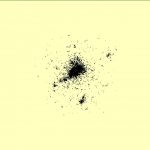
Regarding the latter, consider the paradoxical inward/outward paradox from the perspective of standard statistical-mechanical entropy, as it was presented in Gautestad and Mysterud (2005) and in Part II of this series of posts. The simulation result above shows fixes from two MRW scenaria; MRW fixes that on one hand are generated from applying step length distribution exponent β = 3 (leading to a relatively constrained fix-to-fix distribution of step lengths) and one the other hand from MRW with β = 2 (default MRW; long distant steps more probable). In short, the result of spatial zooming shows the local density of fixes in the “interior” part of the home range as a function of spatial scale, which equals square root of grid cell area. The environment is set to be homogeneous. Both axes are log-transformed for the sake of stressing the respective scenaria’s power law (scale-free) properties. The local number of fixes equals the number of locations per grid cell, calculated over cells with non-zero abundance of locations (incidence). When the spatial resolution is increased from right to left, the density pr. cell area decreases because the given number of fixes is spread over an increasing number of smaller grid cells, and density is calculated as locations pr. non-empty cell at the scale of the new and smaller cell size.
The spatial space use pattern from the condition β = 3 regards a scenario where the animal has concentrated its space use effort towards finer spatial scales, rather than balancing the effort relatively equally over the total scale range of space use (β = 2). Hence, the β = 3 condition shows a slope close to 2 (fractal dimension, D ≈ 2); filled circles). In other words, half as large cell size (square root finer scale) shows half as many fixes pr. cell. This result verifies that the level of “disorder”; i.e., entropy, is maintained at the same level over a range of spatial resolutions. In other words, when D ≈ 2, the space use system's entropy is both “space-filling” and resolution-independent within the given area extent, and thus complies more closely with standard statistical mechanics (see below).
On the other hand, the non-standard ("paradoxical") property that emerges from β = 2 is shown by the smaller slope of magnitude approximating slope = 1; i.e., D ≈ 1 in statistical fractal terms. In other words, half as large cell size shows the square root of half as many fixes pr. cell. Here, density per non-empty cell is increasing non-trivially relative to the given area unit for density calculation and relative to the classic β = 3 condition. This discrepancy, marked by the Δ character, emerges in local density of locations, and shows how local intensity of habitat use – even in a homogeneous environment – increases in a heterogeneous manner towards finer resolutions.**
This implies that a given total number of locations inside the grid arena is concentrated among a smaller and smaller number of cells as cell size is reduced. Consequently, entropy – lack of information of the animal’s whereabouts – is in entropy terms apparently reduced towards finer resolutions. From this kind of statistical self-organization, finer spatial resolutions are expressing increased order and less entropy! From the perspective of standard statistical mechanics (premise of memory-less, Markovian compliant particles and ensemble of fixes), this pattern is paradoxical.
Then let us leave spatial zooming and return to the first aspect of observation intensity; non-trivial N-dependency, as expressed by the home range ghost equation. Consider space use from the perspective of a given grid cell resolution at scale of c = CSSU and how the observed total area of non-empty cells, I, at this particular scale increases as a function of observation intensity N.

In this case, consider two scenaria; (a) the expectation of I(N) from the standard home range theory, and (b) MRW using default contition β = 2. Under the standard home range theory, it is expected that I is approaching an asymptote, "the true home range area", with increasing N (see the grey line in the Figure to the right). As this asymptote area is approached, the "space-filling" D=2 condition with standard entropy expectation is simultaneously approached. The asymptotic approach towards "true" home range area is in this scenario a small-sample artifact; i.e., a trivial I-dependency on N.
Then compare this function with the default MRW expectation β = 2 and spatial pattern D ≈ 1, using grid cell resolution of CSSU (smaller red square). The home range ghost function for I(N) is paradoxical from standard statistical mechanics, because I within the broad scale range for scale-free space use does not approach an asymptote with increasing observation intensity N, but expands proportionally with the square root of N. Further, the small-N artifact is negligible relative to the standard model. Within practical limits of sampling, the "MRW" line in the Figure for N = c√N does not express an asymptotic approach towards a given home range area.
In order to understand the difference in area expectation between the standard framework and the alternative MRW model, labelled as "Ghost" area in the illustration, we have to invoke the outward/inward concept. Basically, to ensure a model for self-organized D ≈ 1 compliant space use that is compatible with the universal entropy-concept of statistical mechanics, I suggest that I should be considered being a product of two independent aspects of space use calculation; observed I at resolution c = CSSU (Ioutwards) and "hidden" space use at finer resolutions than c (Iinwards). This product is marked by a large red square at a given N. This implies that the scale axis is defined to be an independent system variable, just like the standard three coordinates x,y,z for directions in space are inter-independent.
By increasing the sample size of fixes, N, the additional fixes will in succession either happen to fall in a previously empty grid cell (contributing to increase Ioutwards) or in an already non-empty grid cell (contributing to increase Iinwards), keeping I unchanged from that particular increment in N. Since we in this extended statistical-mechanical system consider the observed space use, I at spatial resolution CSSU, to change proportionally with c√N, at any given (realistic) magnitude of N we have Iinwards= Ioutwards.
In short, what we see from increasing N is an increase of Ioutwards. The finer-grained Iinwards only becomes visible if we increase the observational resolution towards finer scales, c < CSSU, rather than keeping c fixed at c ≈ CSSU. To see the effect from this alternative operation of changing resolution rather than changing N, return your focus to the "zooming" illustration above (density vs. scale)!
In order to ensure compliance with entropy at a fixed observational spatial scale c ≈ CSSU, we thus have
√Iinwards * √Ioutwards = Itotal
For a given magnitude of N and for serially non-autocorrelated fixes, Iinwards and Ioutwards both have a magnitude of square root of Itotal. We then have (in relative terms):
“inward” change of entropy + “outward” change of entropy = -0.5 + 0.5 = 0
where the numbers refer to log-transformed disorder and how it changes relative to finer and coarser scales. Thus, for spatial scale the number -0.5 regards slope for log(1/√(grid cell scale) = -0.5 and the number 0.5 regards slope for log(√(grid cell scale).
In comparison, the entropy relationship for the standard space use model should read “inward” change of entropy equals “outward” change of entropy, and both equals zero. The entropy is thus invariant under change of spatial resolution under this classic model condition. According to the classic system, there is no inward/outward paradox from zooming over a range of grid cell resolutions; i.e., by studying the log-transformed function of density over resolution,
“inward” change of entropy + “outward” change of entropy = 0 + 0 = 0
In this case there is no fine-pixel surprise factor in the form of reduced entropy if the observer is zooming in (within a given area extent), and no non-trivial area expansion with increasing sample size, N.
For the sake of improved realism it should be obvious that two alternative sets of ecological methods need to be developed to study animal space use; one for MRW-like assumptions and one for traditional assumptions. Empirical studies should first (a priori) test which statistical-mechanical framework the given animal adhered to at the given locality and time period, and then apply the proper toolbox for the ecological study.
What is gained is an alternative system description, which in our empirical studies has verified giving a more realistic representation of space use as a function of observation intensity of both kinds (Change of N and change of spatial resolution). Consequently, ecological methods that have begun to emerge from this theory produce less noisy correlations; e.g., with respect to habitat selection. I refer to other posts in my blog, and of course my papers and my book.
NOTES
*) "Non-trivial" means that the relationship between N and I is not a small-sample artifact, but qualitatively different and tied to what here is defined as observation intensity. Serially non-auto-correlated fixes are assumed (In a previous post I have described a method that makes the home range ghost formula compatible also with autocorrelated fixes). How the model behaves under heterogeneous environments in space and time have been laid out in detail in other blog posts.
**) The transition towards a common log-log slope of 2 at the coarsest resolutions for both scenaria is an artifact from choosing a grid extent that does not cover the total set of relocations in the given set (i.e., some parts of the distribution at the fringes of the home range were left out, for the sake of studying the home ranges’ “interior”). This effect could, to a large extent, have been avoided by choosing an area extent that covered all fixes.
REFERENCES
Evans, M. R., S. N. Majumdar, and G. Schehr. 2019. Stochastic Resetting and Applications. arXiv:1910.07993v1 [cond-mat.stat-mech].
Gautestad, A. O. and I. Mysterud. 2005. Intrinsic scaling complexity in animal dispersion and abundance. The American Naturalist 165:44-55.