Follow-up on the KDE’s Sample Size Paradox
In a previous post I showed how the combination of scale-free movement and spatial memory utilization generates space use that is incompatible with statistical descriptors under the KDE approach. In short, I advocated that the home range – as observed from the scatter of relocation data (fixes) – should be described by methods that are in better coherence with the underlying process in statistical-mechanical terms. The KDE does not comply with scale-free movement, since the emerging fix scatter is a statistical fractal with dimension D≈1, which makes space use incompatible with a density “surface” (utilization distribution, UD). In the present post I elaborate on this issue, and provide further simulation explorations.
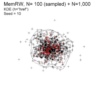
 The illustration to the right shows a home range with a “well-behaved” space use – in close compliance with standard KDE assumptions. The model animal moves scale-specifically (Markov compliant, here represented by correlated random walk), in combination with occasional return events to previously visited locations. In the Scaling cube ((Archive: "The scaling cube". Posted December 25, 2015), this model satisfies the MemRW universality class. The simulated movement path is then sampled at sufficiently large intervals to ensure non-autocorrelated fixes (I will return to autocorrelated series in later posts, where I discuss the Brownian bridge variant of KDE).
The habitat in the present example is homogeneous in order to disentangle the space use effect from intrinsic behaviour from the added effect from habitat heterogeneity (the general argument for homogeneous environment was given in a previous post).
According to MemRW theory, one should expect ca (1000/100)0.25 = 3.2% smaller area demarcation for N=100 relative to N=1,000, since N-dependency is weak; Area ∝ N0.25 (area measured as incidence, see Gautestad et al., 2013). Two sample sizes are superimposed in the illustration above; N=100 (red crosses) and N=1,000. The respective 99% isopleths are quite similar but area from N=100 is ca 10% smaller. It indicates KDE’s ability to almost compensate for the trivial sample size artifact that small samples of fixes tend to show smaller home range areas. The net discrepancy seen here in this “quick and dirty” test is ca (10-100.25)% = 6.8%. Proper small-N compensation from KDE depends on the assumption that the process is scale-specific, as it is in this example.
 What about habitat heterogeneity? The home range to the right shows an example. Habitat heterogeneity is simulated in a simplistic manner, by randomly placing 10 initial start locations for the animal to choose from when accessing its memory map of previously visited locations during return events. The seed locations may be interpreted as a priori preferred patches, for example due to expectation of a particularly high foraging success at these localities, or patch attributes that satisfy the given animal’s habitat preference better than the surrounding area. Due to the MemRW condition (“denser” UD due to a larger fractal dimension, D), this initial set of “preferred patches” is not sufficiently influential to produce strong multi-modality. Other specifications of habitat heterogeneity could have produced stronger modality, though. The 95% isopleth for N=1,000 is also in this example ca 10% larger than the N=100 isopleth. In other words, again a statistically trivial discrepancy relative to expectation, (10-100.25)% = 6.8%.
 Using the same “preferred patches” method under MemRW to impose habitat heterogeneity under scale-free condition (MRW), the initial set of 10 attraction points has a profound effect on modality of the UD. The image to the right shows clear influence from environmental heterogeneity. Thus, the UD from a MRW pattern is more “sensitive” to even subtle levels of environmental heterogeneity, relative to a scale-specific process like MemRW.
For a MRW process, theory predicts Area ∝ N0.5 (area measured as incidence, see Gautestad and Mysterud, 2010, or this post). Contrary to the “well-behaved” MemRW space use above, the MRW model with habitat heterogeneity confirms the KDE paradox: the 99% isoplets N=100 demarcates ca 15% larger area in comparison to N=1,000. The discrepancy is even larger for narrower isopleths, e.g. 90% (N=100 produce ca 30% larger area than N=1,000; not shown). Hence, the total discrepancy under the 99% isopleth is (15+100.5)%=18.2%. Despite the strong multi-modal effect on the UD from adding heterogeneity the result on home range demarcation is quite similar to the same model in a homogeneous environment, as was shown in the previous post.
In other words, the KDE sample size paradox – as found both in empirical studies and in the present theoretical pilot tests on MRW – seems to be quite resilient to environmental conditions. On the other hand, the classic space use condition for home range simulations (here represented by MemRW) behaves in better compliance with statistical expectations, in this case KDE assumptions.
To conclude, also these preliminary tests seem to support scale-free MRW over scale-specific MemRW as model representation for memory-influenced movement, due to their closer compliance with real data’s statistical properties (the KDE paradox). What appears as a statistical paradox under Markov conditions for space use in fact represents a model prediction under the parallel processing conditions (MRW).
REFERENCES
Gautestad, A. O., L. E. Loe, et al. (2013). Inferring spatial memory and spatiotemporal scaling from GPS data: comparing red deer Cervus elaphus movements with simulation models. Journal of Animal Ecology 82(3): 572-586.

The habitat in the present example is homogeneous in order to disentangle the space use effect from intrinsic behaviour from the added effect from habitat heterogeneity (the general argument for homogeneous environment was given in a previous post).
According to MemRW theory, one should expect ca (1000/100)0.25 = 3.2% smaller area demarcation for N=100 relative to N=1,000, since N-dependency is weak; Area ∝ N0.25 (area measured as incidence, see Gautestad et al., 2013). Two sample sizes are superimposed in the illustration above; N=100 (red crosses) and N=1,000. The respective 99% isopleths are quite similar but area from N=100 is ca 10% smaller. It indicates KDE’s ability to almost compensate for the trivial sample size artifact that small samples of fixes tend to show smaller home range areas. The net discrepancy seen here in this “quick and dirty” test is ca (10-100.25)% = 6.8%. Proper small-N compensation from KDE depends on the assumption that the process is scale-specific, as it is in this example.


For a MRW process, theory predicts Area ∝ N0.5 (area measured as incidence, see Gautestad and Mysterud, 2010, or this post). Contrary to the “well-behaved” MemRW space use above, the MRW model with habitat heterogeneity confirms the KDE paradox: the 99% isoplets N=100 demarcates ca 15% larger area in comparison to N=1,000. The discrepancy is even larger for narrower isopleths, e.g. 90% (N=100 produce ca 30% larger area than N=1,000; not shown). Hence, the total discrepancy under the 99% isopleth is (15+100.5)%=18.2%. Despite the strong multi-modal effect on the UD from adding heterogeneity the result on home range demarcation is quite similar to the same model in a homogeneous environment, as was shown in the previous post.
In other words, the KDE sample size paradox – as found both in empirical studies and in the present theoretical pilot tests on MRW – seems to be quite resilient to environmental conditions. On the other hand, the classic space use condition for home range simulations (here represented by MemRW) behaves in better compliance with statistical expectations, in this case KDE assumptions.
To conclude, also these preliminary tests seem to support scale-free MRW over scale-specific MemRW as model representation for memory-influenced movement, due to their closer compliance with real data’s statistical properties (the KDE paradox). What appears as a statistical paradox under Markov conditions for space use in fact represents a model prediction under the parallel processing conditions (MRW).
REFERENCES
Gautestad, A. O., L. E. Loe, et al. (2013). Inferring spatial memory and spatiotemporal scaling from GPS data: comparing red deer Cervus elaphus movements with simulation models. Journal of Animal Ecology 82(3): 572-586.