The Mysterious Taylor’s Power Law – Part IV
Time to verify theoretical coherence between scale-free population abundance and scale-free space use at the individual level! In this part IV of the Taylor law presentation I analyze a simulated set of GPS fixes rather than studying population abundance. In other words, how does the variance-mean relationship in local density of fixes from the multi-scaled random walk model (MRW) resemble V(M) in a local population under the Zoomer model condition? Through the history spanning more than 1,000 papers this acid test has never previously been successfully performed. My presentation also illustrates the so-called Z-paradox, and how it is resolved under the parallel processing framework for animal space use.
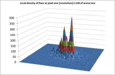 The illustration to the right shows the spatial “home range” scatter from a model individual complying with the MRW model. The number of fixes pr. grid cell of resolution k=1:128 (128×128 cells within the defined arena) shows the commonly observed multi-modal utilization distribution. In this case, and in compliance with all our empirical tests on real data, the distribution is self-similar (fractal), with fractal dimension D≈1.
As described in Chapter 7 of my book, V(M) analysis of fixes shows compliance with Taylor’s power law V=aMb with power exponent b≈2. The illustration below – with log-transformed data – shows “transects” of local fix abundance at various spatial resolutions (see Note below). For example, the red dots illustrate V(M) at resolution k=1:128 relative arena size k≡1, where each dot is a given V(M) pair in the “red” set of 128 transect rows. The blue dots show the similar set of transects at resolution 1:64, and so on towards coarser spatial scales 1:32, 1:16 and 1:8. The black dots with regression line show the over-all V(M) for all grid cells at respective resolutions, instead of splitting the cells into transects at respective scales.
 According to standard, “well-behaved” statistics (Poisson-compliant, where b=1), one should expect the black V(M) series to overlap the transect sets. In other words, the intercept log(a) should be similar when studying V(M) at a coarse resolution. In short, the variance of the total set equals the sum of the variance of the parts. Why this is not true here in the context of complex (scale-free) space use, is previously explained as the Z-paradox. This paradox emerges when the classical theory for variance is applied on non-classical space use. By applying the parallel processing theory the paradox is resolved, as shown below!
 By multiplying the variance for each V(M) pair with a scale-dependent coefficient equal to the square root of 1/k (so-called rescaling), we get full compliance between mean and variance at respective scales when the V(M) sets from respective scales are superimposed. In other words, this rescaling is represented by the coefficient a in Taylor’s power law under the present model conditions where we study cross-scale scaling of parallel processing-compliant space use at the individual level. The magnitude of a in this context increases with the relative scale range when comparing V(M) at different resolutions. For example, for k = 1/128 we have a = √128 = 11.31. Thus, log(a) = 1.05, which is very close to the y-axis intercept log(a) = 0.90 that was calculated for the log(V,M) regression at the chosen reference scale k≡1 in the pilot test above (black dots).
Why square root? Because b=2 implies that the standard deviation (SD), which equals the square root of V, is proportional with the mean, M. Thus, the present statistical-mechanical framework implies that its V(M) statistics are compliant with the properties of a Cauchy distribution (Lévy stable distribution of index 1) rather than the normal Gaussian under which variance is proportional with the mean.
The illustrative result above comes from a single set of GPS fixes. If the procedure had been replicated, the average V(M) scatter from respective replicates would in the limit of large number of replicates show less scatter around the regression line.
From a statistical-mechanical perspective this result verifies coherence between time average and ensemble average of space use by a “particle” or a set of particles, but hereby – for the first time to my knowledge – from the context of a complex (scale-free) process with b>>1.
GPS fixes from MRW represent the time evolution of a single particle’s space use (in statistical terms), and the ensemble average from the Zoomer model shows a population of particles’ space use at a given point in time (after some initial evolution of implicit individual movement).
For the first time a statistical-mechanical framework is able to show coherence between individual level and population level dynamics in the context of V(M) statistics, in compliance with Taylor’s power law and thus a broad range of empirical data. In technical terms, the dual-level MRW/Zoomer model simulates a so-called Lévy-stable process (Mandelbrot 1983) over a scale range. Hence, hereby the theoretical regime of statistical fractals is connected to Taylor’s power law through novel extensions of standard (Markov-compliant and scale-specific) statistical-mechanics!
In the next part of this series I will illustrate Taylor’s power law and its scale-free property using my own empirical data on a local population of aphids.
NOTE
In compliance with Hanski (1982) I have adjusted for small-sample artifacts by modifying Taylor’s law to V = aMb + M. This modification was not performed in my book’s presentation of the same data (Figure 43).
REFERENCES
Hanski, I. 1982. On patterns of temporal and spatial variation in animal populations. Ann. zool. Fermici 19: 21—37
Mandelbrot, B. B. 1983. The fractal geometry of nature. New York, W. H. Freeman and Company.
As described in Chapter 7 of my book, V(M) analysis of fixes shows compliance with Taylor’s power law V=aMb with power exponent b≈2. The illustration below – with log-transformed data – shows “transects” of local fix abundance at various spatial resolutions (see Note below). For example, the red dots illustrate V(M) at resolution k=1:128 relative arena size k≡1, where each dot is a given V(M) pair in the “red” set of 128 transect rows. The blue dots show the similar set of transects at resolution 1:64, and so on towards coarser spatial scales 1:32, 1:16 and 1:8. The black dots with regression line show the over-all V(M) for all grid cells at respective resolutions, instead of splitting the cells into transects at respective scales.


Why square root? Because b=2 implies that the standard deviation (SD), which equals the square root of V, is proportional with the mean, M. Thus, the present statistical-mechanical framework implies that its V(M) statistics are compliant with the properties of a Cauchy distribution (Lévy stable distribution of index 1) rather than the normal Gaussian under which variance is proportional with the mean.
The illustrative result above comes from a single set of GPS fixes. If the procedure had been replicated, the average V(M) scatter from respective replicates would in the limit of large number of replicates show less scatter around the regression line.
From a statistical-mechanical perspective this result verifies coherence between time average and ensemble average of space use by a “particle” or a set of particles, but hereby – for the first time to my knowledge – from the context of a complex (scale-free) process with b>>1.
GPS fixes from MRW represent the time evolution of a single particle’s space use (in statistical terms), and the ensemble average from the Zoomer model shows a population of particles’ space use at a given point in time (after some initial evolution of implicit individual movement).
For the first time a statistical-mechanical framework is able to show coherence between individual level and population level dynamics in the context of V(M) statistics, in compliance with Taylor’s power law and thus a broad range of empirical data. In technical terms, the dual-level MRW/Zoomer model simulates a so-called Lévy-stable process (Mandelbrot 1983) over a scale range. Hence, hereby the theoretical regime of statistical fractals is connected to Taylor’s power law through novel extensions of standard (Markov-compliant and scale-specific) statistical-mechanics!
In the next part of this series I will illustrate Taylor’s power law and its scale-free property using my own empirical data on a local population of aphids.
NOTE
In compliance with Hanski (1982) I have adjusted for small-sample artifacts by modifying Taylor’s law to V = aMb + M. This modification was not performed in my book’s presentation of the same data (Figure 43).
REFERENCES
Hanski, I. 1982. On patterns of temporal and spatial variation in animal populations. Ann. zool. Fermici 19: 21—37
Mandelbrot, B. B. 1983. The fractal geometry of nature. New York, W. H. Freeman and Company.