MRW and Ecology – Part II: Space Use Intensity
Through the history of ecological methods, local intensity of habitat use has been equalized with local density of relocations. Using relative density as a proxy variable for intensity of habitat use rests on a critical assumption which few seems to be aware of or pay attention to. In this second post on Multi-scaled random walk (MRW) applications for ecological inference I describe a simple method, which rests on an alternative assumption with respect to space use intensity, applicable under quite broad behavioural and ecological conditions. One immediate proposal for application is analysis of habitat selection.
First, consider counting number of GPS fixes, N, within respective area segments of a given habitat type h, Ah1, Ah2, …, Ahi, …Ahk, and calculating the average N pr. area unit of type h. Next, consider comparing this density Dh with another density within a second habitat type j; i.e., Dj, using the same area scale for comparison. If Dh>Dj one traditionally assumes that the intensity of use of habitat h has been stronger than habitat j. Ecological inference about habitat selection then typically follows under this assumption. In the following I describe the critical assumption for applicability of this traditional method, and I conclude with an alternative proxy variable.
The assumption that space use intensity can be represented by density of space use rests on a specific statistical-mechanical property of particle movement. In our context, the particle is an individual.
The concept of space use intensity in ecology may be represented by local particle density of relocations if – and only if – the particle follows the physics of a Markovian process, and the particle has no affinity towards previously visited locations.
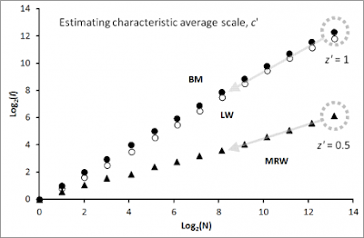 Why? Consider the simulation result to the right, where a particle has moved in compliance with a classical random walk (Brownian motion-like; filled circles) and a Lévy walk (open circles). In both instances the number of pixels (“virtual grid squares”, I, at respective unit process scales) that embed at least one relocation of the particle grows proportionally with N. This property of proportionality applies both to the present condition where N represents the entire path of the particle – meaning that N grows in proportion to path length – and an alternative condition where the path is sampled at larger intervals than the given unit time scale, t. In short, at the unit spatial scale and the complementary unit temporal scale t, every new step tends to hit a previously non-visited pixel. Since each displacement at this dual space-time scale is independent of previous steps (the Markov condition) and every path crossing happens by chance (the independence of previous locations condition), dividing N by total area visited, N/I ≡ D, gives a constant density value. If the environment is spatially heterogeneous (“habitat heterogeneity”, as illustrated by the types h and j above), the local density will vary accordingly.
In other words, under this specific and quite restrictive condition intensity of space “use” is equal to density of space use. If the respective unit process scales were changed, D would also change proportionally (recall from above, that respective D-estimates should be compared under a similar spatial scale; i.e., same pixel size). Hence, in an ecological context habitat selection could be inferred by studying difference in density under assumed different characteristic scales for the movement process as the animal passes through respective types of habitat.
Then consider the widespread condition where an animal’s path is not self-crossing by chance only, due to some degree of affinity to previously visited locations in a manner that - consequenyly - is not compatible with a Markovian process. In ecology we call it a home range compliant kind of space use (the home range becomes and emergent property from site fidelity).
Under this condition, density should not be applied as a proxy variable for local intensity of space use. You should be critical to the fact that more than 99% of researchers disregard this piece of advice in situations where the individual has shown home range behaviour in an obvious non-Markovian manner! Misuse of D as a proxy for intensity will clearly inflate the error term substantially in ecological use-availability analyses. I’m happy to see that this fact finally starts percolating into basic models of space use data (Campos et al. 2014; Morellet et al 2013). Downplaying the density-intensity issue by applying kernel density or Brownian bridge representations of local D estimates will not resolve the challenge. These methods also rest on the same classical assumption as described above. Garbage in – garbage out!
As all readers of my book and my blog are aware of, I advocate MRW as a more realistic substitute. The result marked by MRW (filled triangles) in the Figure above shows how I increases proportionally with the square root of N (log-log slope z=0.5); i.e., a non-proportional and very “dampened” expansion of I relative to the classical condition of Brownian motion and Lévy walk.
As a consequence, average intensity of space use in respective habitat types should be represented by D’ = (√N)/I, not by D = N/I. According to the MRW theory, D’ = 1/c, where c is the actual MRW process’ characteristic scale. The exploratory part of MRW is per se scale-free (like Lévy walk), but the site fidelity part of the model behaviour introduces a the particular scale c (I refer the reader to a multitude of previous posts on this theme, or to my book).
 The histogram above shows local density (N pr. grid cell = D) of fixes (left pane) and local c of simulated MRW path in a homogeneous environment (Gautestad, in prep.). Since the environment is homogeneous in this scenario, the expectation is c of same magnitude in all grid cells, regardless of local density of fixes. Within each grid cell, c is estimated from the function I(N) = c√N (“The home range ghost” formula), where I is the chosen pixel size within each cell. Contrary to local D estimates, and despite a very crude and simple first-approach method to estimate of local c, the respective columns are quite concentrated around the average c score for the arena as a whole (dotted blue level.
 As shown to the right, local D and c estimates are shown to be independent. While local D in this homogeneous scenario varies tremendously (x-axis shows N pr. grid cell), c varies within a relatively restricted range. Observe that in this regression of c(N), the superimposed text “Dstep = 1″ refers to the fractal dimension of the movement path.
In a previous post I showed by example how the estimate of c can be further improved by fine-tuning the pixel resolution (unit scale for I) for respective grid cell samples of fixes. In the present illustration, pixel size was constant and a priori set somewhat smaller than the given characteristic c = (2 length units)2 = 4 area units. In other words, the pixel scale was set to 1/4 of true c. Still the estimated average c = 21.8 = 3.4 times larger than pixel size, which is close to the true c = 4 area units in over-all terms. Choosing a smaller pixel scale a priori than the true unit scale may explain some deviance from the expected constancy of I in some grid cells (in particular in cells with N ≈ 24).
Additional methodological details: search Archive for "Towards an Alternative Proxy for Space Use Intensity".
In a follow-up post I’ll show the influence of serial auto-correlation in the set of fixes, and how it can be accounted for when using 1/c as an alternative – and more realistic – proxy variable for local intensity of space use. A very nagging problem under the present paradigm may be resolved with ease under the MRW statistical-mechanical model assumptions!
REFERENCES
Campos, F. A., M. L. Bergstrom, A. Childers, J. D. Hogan, K. M. Jack, A. D. Melin, K. N. Mosdossy et al. 2014. Drivers of home range characteristics across spatiotemporal scales in a Neotropical primate, Cebus capucinus. Animal Behaviour 91:93-109.
Morellet, N., C. Bonenfant, L. Börger, F. Ossi, F. Cagnacci, M. Heurich, P. Kjellander et al. 2013. Seasonality, weather and climate effect home range size in roe deer across a wide latitudinal gradient within Europe. Journal of Animal Ecology 82:1326-1339.
First, consider counting number of GPS fixes, N, within respective area segments of a given habitat type h, Ah1, Ah2, …, Ahi, …Ahk, and calculating the average N pr. area unit of type h. Next, consider comparing this density Dh with another density within a second habitat type j; i.e., Dj, using the same area scale for comparison. If Dh>Dj one traditionally assumes that the intensity of use of habitat h has been stronger than habitat j. Ecological inference about habitat selection then typically follows under this assumption. In the following I describe the critical assumption for applicability of this traditional method, and I conclude with an alternative proxy variable.
The assumption that space use intensity can be represented by density of space use rests on a specific statistical-mechanical property of particle movement. In our context, the particle is an individual.
The concept of space use intensity in ecology may be represented by local particle density of relocations if – and only if – the particle follows the physics of a Markovian process, and the particle has no affinity towards previously visited locations.

In other words, under this specific and quite restrictive condition intensity of space “use” is equal to density of space use. If the respective unit process scales were changed, D would also change proportionally (recall from above, that respective D-estimates should be compared under a similar spatial scale; i.e., same pixel size). Hence, in an ecological context habitat selection could be inferred by studying difference in density under assumed different characteristic scales for the movement process as the animal passes through respective types of habitat.
Then consider the widespread condition where an animal’s path is not self-crossing by chance only, due to some degree of affinity to previously visited locations in a manner that - consequenyly - is not compatible with a Markovian process. In ecology we call it a home range compliant kind of space use (the home range becomes and emergent property from site fidelity).
Under this condition, density should not be applied as a proxy variable for local intensity of space use. You should be critical to the fact that more than 99% of researchers disregard this piece of advice in situations where the individual has shown home range behaviour in an obvious non-Markovian manner! Misuse of D as a proxy for intensity will clearly inflate the error term substantially in ecological use-availability analyses. I’m happy to see that this fact finally starts percolating into basic models of space use data (Campos et al. 2014; Morellet et al 2013). Downplaying the density-intensity issue by applying kernel density or Brownian bridge representations of local D estimates will not resolve the challenge. These methods also rest on the same classical assumption as described above. Garbage in – garbage out!
As all readers of my book and my blog are aware of, I advocate MRW as a more realistic substitute. The result marked by MRW (filled triangles) in the Figure above shows how I increases proportionally with the square root of N (log-log slope z=0.5); i.e., a non-proportional and very “dampened” expansion of I relative to the classical condition of Brownian motion and Lévy walk.
As a consequence, average intensity of space use in respective habitat types should be represented by D’ = (√N)/I, not by D = N/I. According to the MRW theory, D’ = 1/c, where c is the actual MRW process’ characteristic scale. The exploratory part of MRW is per se scale-free (like Lévy walk), but the site fidelity part of the model behaviour introduces a the particular scale c (I refer the reader to a multitude of previous posts on this theme, or to my book).


In a previous post I showed by example how the estimate of c can be further improved by fine-tuning the pixel resolution (unit scale for I) for respective grid cell samples of fixes. In the present illustration, pixel size was constant and a priori set somewhat smaller than the given characteristic c = (2 length units)2 = 4 area units. In other words, the pixel scale was set to 1/4 of true c. Still the estimated average c = 21.8 = 3.4 times larger than pixel size, which is close to the true c = 4 area units in over-all terms. Choosing a smaller pixel scale a priori than the true unit scale may explain some deviance from the expected constancy of I in some grid cells (in particular in cells with N ≈ 24).
Additional methodological details: search Archive for "Towards an Alternative Proxy for Space Use Intensity".
In a follow-up post I’ll show the influence of serial auto-correlation in the set of fixes, and how it can be accounted for when using 1/c as an alternative – and more realistic – proxy variable for local intensity of space use. A very nagging problem under the present paradigm may be resolved with ease under the MRW statistical-mechanical model assumptions!
REFERENCES
Campos, F. A., M. L. Bergstrom, A. Childers, J. D. Hogan, K. M. Jack, A. D. Melin, K. N. Mosdossy et al. 2014. Drivers of home range characteristics across spatiotemporal scales in a Neotropical primate, Cebus capucinus. Animal Behaviour 91:93-109.
Morellet, N., C. Bonenfant, L. Börger, F. Ossi, F. Cagnacci, M. Heurich, P. Kjellander et al. 2013. Seasonality, weather and climate effect home range size in roe deer across a wide latitudinal gradient within Europe. Journal of Animal Ecology 82:1326-1339.