A Statistical-Mechanical Perspective on Site Fidelity – Part V
Two important statistical-mechanical properties need to be connected to the home range concept under the parallel processing postulate; micro- and macrostates. When a system is in its equilibrium state, (a) all microstates are equally probable and (b) the observed macrostate is the one with the most microstates. The equilibrium state implies that entropy is maximized.
First consider a physical system consisting of indistinguishable particles. For example, in a spatially constrained volume G of gas (a classical, non-complex system) that consists of two kinds of molecules, at equilibrium you expect a homogeneous mixture of these components. At every virtually defined locality g within the volume, the local density (N/g) of each type of molecule is expected to be the same, independently of the resolution of the two- or three-dimensional virtual grid cell g we use to test this prediction.
This homogeneous state is in compliance with a prediction based on the most probable macrostate for N particles, due to the system’s equilibrium condition. Entropy is the same everywhere within our system, both when comparing localities at a given resolution g within G, and when comparing entropy at different resolutions. In the latter case, the coarser-scale entropy is a simple sum of the entropy of the embedded grid cells at finer cell sizes. However, these properties and linear relationships require “Markov-compliant” dynamics at micro-resolutions (see Preface of my book, or previous posts). In this post I describe the statistical-mechanical micro-/macrostate concepts from the classical home range model’s perspective (the convection model; see previous posts), which satisfies this Markov assumption.
The description below thus serves as a preparation for a follow-up posts in this series, where I intend to present properties with respect to micro-/macrostates under the non-Markovian condition for complex space use; i.e., under the premise of parallel processing. One can then compare classic system properties as they are generally assumed in statistical analysis of animal space use, with the alternative set of properties under the parallel processing conjecture.
Hence, first consider the standard statistical-mechanical description, based on a series of N serially non-autocorrelated fixes from an individual’s movement within its home range. This implies that the condition of a “deep” hidden layer is satisfied, meaning that the data may be interpreted in the context of statistical mechanics.
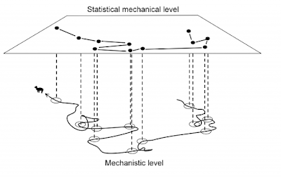 The image to the left illustrates how the hidden layer emerges from sampling an animal’s path in the serially autocorrelated domain. This condition implies that ergodicity is satisfied only at relatively fine resolutions g within G, not at the scales of the path as a whole as represented by G (see Part I of this group of posts). To achieve full ergodicity at scale G the sampling interval (lag) should be large enough to make at least one return event probable within this interval. The sampled series would then have reached the non-autocorrelated domain of statistical-mechanical system representation.
Let us in the following assume this coarser range of temporal sampling scales. At this fully expressed ergodic condition of space use at the home range scale G, the micro/macrostate aspects of a complex home range process may most easily be compared to classic predictions. In this state the animal’s present location gives no indication of its next location within the home range. The utilization distribution (UD, the “density surface of fixes”) is then expected – due to the unpredictability of the animal’s next location based on the present location – to properly reflect the spatially varying probability of the next fix’ actual location.
Simply stated, this probability function – whether simple 2-dimensional Gaussian distribution or a more complicated but realistic multi-modal form (reflecting intra-home range habitat heterogeneity) is the most probable outcome from N fixes, given that N is very large. Why? The answer requires a statistical-mechanical system description. Thus, let us superimpose a virtual grid onto the spatial scatter of N fixes.
Respective grid cells of size g have local density of fixes varying from zero to (quite unlikely) the theoretical maximum N within the given set of cells. Then consider one of these cells, with density N’/g, where g is grid cell area at the chosen resolution. Since we assume a classical system, N’ represents the collection of mutually independent revisit events to this cell during the total sampling time T.
In that respect, one aspect that may of you may find outright disturbing is my argument that the floor of the illustration above under a broad range of annimal space use conditions should not be termed “mechanistic” . Because parallel processing violates the Markovian principle, which represents the foundation both for a mechanistic process and its statistical-mechanical representation, the lower level needs to be renamed and the upper level will need an extended theory.
I call the process non-mechanistic, which is quite different from “static”. It means a generalized form of dynamics, where mechanistic behaviour is embedded as a special case where the process complies with the Markovian principle.
First consider a physical system consisting of indistinguishable particles. For example, in a spatially constrained volume G of gas (a classical, non-complex system) that consists of two kinds of molecules, at equilibrium you expect a homogeneous mixture of these components. At every virtually defined locality g within the volume, the local density (N/g) of each type of molecule is expected to be the same, independently of the resolution of the two- or three-dimensional virtual grid cell g we use to test this prediction.
This homogeneous state is in compliance with a prediction based on the most probable macrostate for N particles, due to the system’s equilibrium condition. Entropy is the same everywhere within our system, both when comparing localities at a given resolution g within G, and when comparing entropy at different resolutions. In the latter case, the coarser-scale entropy is a simple sum of the entropy of the embedded grid cells at finer cell sizes. However, these properties and linear relationships require “Markov-compliant” dynamics at micro-resolutions (see Preface of my book, or previous posts). In this post I describe the statistical-mechanical micro-/macrostate concepts from the classical home range model’s perspective (the convection model; see previous posts), which satisfies this Markov assumption.
The description below thus serves as a preparation for a follow-up posts in this series, where I intend to present properties with respect to micro-/macrostates under the non-Markovian condition for complex space use; i.e., under the premise of parallel processing. One can then compare classic system properties as they are generally assumed in statistical analysis of animal space use, with the alternative set of properties under the parallel processing conjecture.
Hence, first consider the standard statistical-mechanical description, based on a series of N serially non-autocorrelated fixes from an individual’s movement within its home range. This implies that the condition of a “deep” hidden layer is satisfied, meaning that the data may be interpreted in the context of statistical mechanics.

Let us in the following assume this coarser range of temporal sampling scales. At this fully expressed ergodic condition of space use at the home range scale G, the micro/macrostate aspects of a complex home range process may most easily be compared to classic predictions. In this state the animal’s present location gives no indication of its next location within the home range. The utilization distribution (UD, the “density surface of fixes”) is then expected – due to the unpredictability of the animal’s next location based on the present location – to properly reflect the spatially varying probability of the next fix’ actual location.
Simply stated, this probability function – whether simple 2-dimensional Gaussian distribution or a more complicated but realistic multi-modal form (reflecting intra-home range habitat heterogeneity) is the most probable outcome from N fixes, given that N is very large. Why? The answer requires a statistical-mechanical system description. Thus, let us superimpose a virtual grid onto the spatial scatter of N fixes.
Respective grid cells of size g have local density of fixes varying from zero to (quite unlikely) the theoretical maximum N within the given set of cells. Then consider one of these cells, with density N’/g, where g is grid cell area at the chosen resolution. Since we assume a classical system, N’ represents the collection of mutually independent revisit events to this cell during the total sampling time T.
- Microstates: A total of N relocations of the animal implies N-1 time steps of sampling during T, with intervals (“lag”) of length t = T/(N-1) ≈ T/N. Within this range of time scales, from t to T, consider the local series of events in a given grid cell, leading eventually to density N’/g during T. In some extreme cases, the N’ fixes could appear successively from the moment it was observed in the cell for the first time at the n’th increment (0<n<N-N’) and then during each of the following N’-1 observations. In another scenario consider that only N’-1 observations took place in succession, while the last one appearing anytime during the remaining intervals, t, between n=0 and n=N. Each of these combinations represents a given microstate (permutation under a given condition). Hence, the “(N’-1) +1″ set of microstates” is larger and thus more probable than the “N’+0” set of microstates, given that N'<<N. Similarly, an “(N’-2)+2” scenario is more probable than the two foregoing scenaria.
- Macrostate: The scenario with the largest set of microstates is the one that we most likely will find in a local subset of N’ fixes from a total set of N. Under this specific condition we can calculate the system’s entropy as the sum of this maximized magnitude of microstates. If we split the series of GPS fixes into N/x equal parts (x is a positive integer and x<<N), we expect to find N’/x fixes in the given cell, with some statistical variation given by locally varying staying times (a function of the animal’s behaviour and its interaction with the local environment within g). In other words, the local density of fixes is expected to change inversely proportional with x. Hence, the utilization distribution (UD) of the animal’s space use is in this scenario in principle independent of N. However, the larger the sample size the closer we find the estimated UD from N fixes to satisfy the true UD from “infinite” N. The standard error of respective local mean densities over subsets N’/x decreases trivially (square root-kind of change) with increasing N and thus with increasing N’.
In that respect, one aspect that may of you may find outright disturbing is my argument that the floor of the illustration above under a broad range of annimal space use conditions should not be termed “mechanistic” . Because parallel processing violates the Markovian principle, which represents the foundation both for a mechanistic process and its statistical-mechanical representation, the lower level needs to be renamed and the upper level will need an extended theory.
I call the process non-mechanistic, which is quite different from “static”. It means a generalized form of dynamics, where mechanistic behaviour is embedded as a special case where the process complies with the Markovian principle.