Spatial Analysis of Serially Autocorrelated Fixes
In previous posts I have mostly assumed serially non-autocorrelated fixes, and simulations have also reflected this coarse temporal sampling scale. However, in this post I started exploring the autocorrelation effect’s interesting statistical-mechanical properties. In this post I elaborate further on this theme, in particular its enhanced effect on the N-paradox under the kernel density estimation (KDE).
From a statistical-mechanical perspective a high degree of coarse-graining of an animal’s space use is an advantage, due to a deep “hidden layer” and – consequently – better compliance with the ergodic principle in statistical mechanics. In short, system parameters are more precisely estimated when some spatio-temporal scale distance from the animal’s true path is achieved. In practice GPS series are often collected at high frequency in order to give large series for statistical analysis. This is an advantage for detailed ecological inference at the behavioural “micro-scale” of path analysis, but may hinder a proper statistical-mechanical approach towards description of statistical-mechanical system properties. However even in the domain of serially autocorrelated data the statistical-mechanical analysis makes sense, given that the system extent is similarly constrained (spatial range needs to be constrained to reflect finer temporal resolution, and thereby reinstate better compliance with system ergodicity (Archive: search this term).
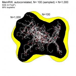 I have previously criticized the KDE for lack of power to distinguish scale-specific from scale-free space use. In the two illustrations to the right I show a similar KDE analysis based on more high-frequently sampled paths, leading to serial autocorrelation. I acknowledge that KDE is strictly meant for non-autocorrelated series. However, since many are applying this approach also for high frequency series I briefly comment on this scenario here.
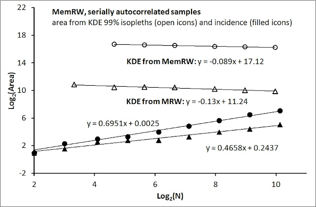
The N-paradox – KDE area becoming larger for small samples of fixes – is clearly visible also for autocorrelated series: a smaller sample tends to show a larger area – yellow colour – for a given 99% isopleth both for scale-specific (MemRW) and scale-free (MRW) movement. Like I found for non-autocorrelated series, the discrepancy is even larger for smaller percentage “slices” of the utilization distribution (not shown). The KDE results for autocorrelated series are shown in the illustration below (open symbols).
 I have previously documented how the KDE is unable to differentiate between a scale-specific and a scale-free kind of space use. Thus, under the condition of scale-free space use (and consequently applying the proposed incidence method – counting non-empty virtual grid cells for a given N – as an alternative to KDE) auto-correlated series require some additional caution with respect to estimate the important MRW parameters c and z. These parameters are estimated from the home range ghost formula for incidence, I(N) = cNz.
Exploration of simulations leads to the following rules-of-thumb:
From a statistical-mechanical perspective a high degree of coarse-graining of an animal’s space use is an advantage, due to a deep “hidden layer” and – consequently – better compliance with the ergodic principle in statistical mechanics. In short, system parameters are more precisely estimated when some spatio-temporal scale distance from the animal’s true path is achieved. In practice GPS series are often collected at high frequency in order to give large series for statistical analysis. This is an advantage for detailed ecological inference at the behavioural “micro-scale” of path analysis, but may hinder a proper statistical-mechanical approach towards description of statistical-mechanical system properties. However even in the domain of serially autocorrelated data the statistical-mechanical analysis makes sense, given that the system extent is similarly constrained (spatial range needs to be constrained to reflect finer temporal resolution, and thereby reinstate better compliance with system ergodicity (Archive: search this term).
The N-paradox – KDE area becoming larger for small samples of fixes – is clearly visible also for autocorrelated series: a smaller sample tends to show a larger area – yellow colour – for a given 99% isopleth both for scale-specific (MemRW) and scale-free (MRW) movement. Like I found for non-autocorrelated series, the discrepancy is even larger for smaller percentage “slices” of the utilization distribution (not shown). The KDE results for autocorrelated series are shown in the illustration below (open symbols).
Exploration of simulations leads to the following rules-of-thumb:
- Incidence (I) should be calculated separately over a range of spatial resolutions (grid scales) to find optimal scale, as outlined in this post. If the data are MRW compliant one should observe that z will tend to increase slightly beyond z=0.5 for small grid scales, and decrease below z=0.5 at larger scales relative to the optimal scale. These tendencies are visible both for non-autocorrelated and autocorrelated series, but is more pronounced in the latter case.
- The best parameter estimates are achieved by applying the grid scale with best compliance with z=0.5 to find c from the intercept at this scale (this is not a tautology, due to extra statistical information that can be extracted from the regressions; I will explain in a later post). The characteristic scale of space use, CSSU, can then be estimated by the simple calculation shown here.
- Observe that CSSU is dependent on sampling frequency when data are autocorrelated. Thus, CSSU is time-dependent under this condition. A modifying factor is thus needed to correct for the strength of autocorrelation. See explanation in a previous post. However, also for this condition I provide a solution in an upcoming post.
- If the underlying process is not MRW compliant but both scale-specific an serially auto-correlated (illustrated below by the MemRW with a z=0.69 estimate; filled circles), the incidence approach is apparently non-consistent with the expected z = 0.25 which was previously shown for non-autocorrelated sampling. The reason for the large discrepancy of z in this particular scenario is easy to explain. At a the fine-grained sampling scale in the domain of autocorrelation a 2-speed movement is revealed under the present conditions (instantaneous relocation during a return event, like a ground-foraging bird with sudden return flights to a previous patches). This speed variability is “hidden” if sampling interval is increased relative to the present autocorrelated fixes, and thereby achieving non-autocorrelated series from sub-sampling. Consequently, z=0.25 should then be expected to be maintained also for this type of 2-speed movement – as was in fact documented in the previous post. In other words, the inflated z in the result below for MemRW is due to interference from path dynamics at fine resolutions into the “hidden layer” scales, leading to an intermittent process between micro- and meso-scale dynamics. Thus, z=0.69 is a statistical artifact – a curiosity – from this mixture of movement modes at the chosen observation frequency of fixes.
