Simulating Populations I: the Bridge Towards Standard CML
My book’s title reads: “Animal Space use: Memory Effects, Scaling Complexity, and Biophysical Model Coherence“. The latter part refers in particular to model compliance between individual- and population-level dynamics in spatially extended systems. Within the standard statistical-mechanical framework there is a well-developed theory for such coherence, based on memory-free and non-scaling (Markov-compliant) dynamics. However, as my book and blog is highlighting, the standard approaches towards modelling animal space use are often struggling when validated against high-quality spatio-temporal data. In a series of posts I illustrate challenges and potential solutions at the population level by exploring the Zoomer model – a parsimonious variant of the individual level Multi-scaled random walk model.
First, I want to recap a citation from a previous post:
“Parsimonious models are simple models with great explanatory predictive power. They explain data with a minimum number of parameters, or predictor variables. The idea behind parsimonious models stems from Occam’s razor, or “the law of briefness” (sometimes called lex parsimoniae in Latin). The law states that you should use no more “things” than necessary; In the case of parsimonious models, those “things” are parameters. Parsimonious models have optimal parsimony, or just the right amount of predictors needed to explain the model well.”
http://www.statisticshowto.com/parsimonious-model/
A parsimonious model is the natural starting point when stepping away from the standard methods. By exploring a system’s behaviour at its very basic level, the core properties may be compared and tested against an alternative framework. Later on, additional layers of details may then be successively added to the basic model, for the sake of improved realism and case-specific tailor-making.
I have already described the Zoomer model’s basic properties in a range of posts (Archive: search for “Zoomer model”). A more detailed walk-through is provided in my book. Below I spin a thread from the Zoomer model towards the standard approaches of spatio-temporal population dynamics by tuning the simulation condition towards a scale-specific and memory-less variant. In short: I switch off zooming (multi-scaled space use), and achieves a standard and parsimonious coupled map lattice (CML) model. This presentation then represents the entry point towards the extended system to be explored in the follow-up posts.
For the sake of exploring the populations’ intrinsic and most basic space use behaviour (prior to studying their responses to environmental heterogeneity and perturbations) I define a condition of a homogeneous environment. Generally I also go for a high frequency time axis, to underscore the fact that individual reshuffling generally has a more volatile effect on population dispersion of non-sessile animals than intrinsic death and growth rates.
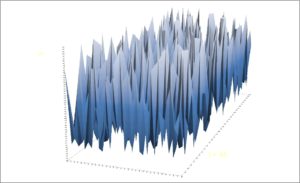 Scenario 1. First, consider an extreme case of spatially extended “boom and bust” dynamics, as illustrated to the left (local density at the z-axis). The CML scenario describes a 32×32 cell arena where individuals show strong local reproduction and weak local survival during a time increment (survival rate: 0.6; reproduction rate: 0.5, net growth 0.1). When a local population reaches the defined carrying capacity*, on average 90% of the individuals are emigrating or dying. In other words, 90% of the emigrants are redistributing themselves randomly within the arena, and the rest are either leaving the arena or dying. image below shows a transect of local population density, and the bottom image presents a multi-scaled snapshot of
 log(mean number of individuals) versus log(variance) of transects at respective spatial resolutions.
In the present context, the mean M is calculated in a rather non-conventional manner by summing individuals over local groups of cells (coarse-graining local density), and plotting the respective scales’ log(M,V) results in the same graph. In this manner the population’s variability characteristics are visualized over a scale range. In other words, M is proportional with the degree of spatial coarse-graining.
 In this example, the variance is strong (V >> M), and V varies approximately proportionally with M (and thus with spatial scale in this plot). This is indicative of an exponential distribution of local population density, which is to be expected due to the “boiling” boom and bust condition.
Scenario 2. What if the population as a whole for most of its local parts are some distance from reaching the actual carrying capacity? Recall from standard ecological theory that local populations that are subject to relative (percent-wise) fluctuations – like variability in growth rate – are expected to show a log-normal distribution with V∝M2.
 The latter scenario is shown to the left, using the same carrying capacity (however, at the present point in time the population density is relatively low and thus not influence by it), and with more subdued dynamics than in the first example: local overshoot emigration reduced from 90% to 50%. Further, local populations are dynamically coupled by a two-dimensional diffusion rate of 2% pr. time increment, which represents random immigration and emigration (two-way reshuffling) to a given cell during a given time increment.
 Diffusion tends to “smoothen” the total population’s density surface by introducing strong spatial auto-correlation, which is clearly visible in both the density surface and the transect snapshot to the left. Further, diffusion – like local growth and birth rate – influences local density in a relative manner and thus supporting a log-normal distribution with V∝M2, as shown in the lower image. Since the current process is defined to be scale-specific due to using a standard model framework (we are accepting a CML model to represent it and we are using diffusion for local re-shuffling, right?), diffusion to more distant cells during one time increment can be ignored if neighbour cell diffusion is small. In the present example, next-nearest neighbour diffusion rate is 0.02*0.02=0.0004, or 0.04%.
 The dynamics of both scenaria are basic stuff for population dynamical modelling, and solidly explored under standard CML designs. The two process variants are also well understood within the complementary standard statistical mechanical theory. In particular, the respective log(M,V) plots provide on one hand the expected characteristics of a system satisfying ergodicity (first scenario above; V ≈ aM, spatially non-autocorrelated) and on the other hand a linear local coupling leading to spatial autocorrelation and V≈aM2 due to diffusion and most or all local populations below the carrying capacity (second scenario above; ergodicity only satisfied within grid cells). For an ergodic system one expects a power exponent ß≈1 [slope ≈ 1 as in the uppermost log(M,V) plot], while autocorrelation leads to 1< ß <≈ 2, and limits population ergodicity to fine scales.
 Scenario 3. Another characteristic property of a scale-specific process is the tendency even for conditions leading to autocorrelation with ß ≈ 2 (in practice, in the range 1.3 < ß < 1.8 due to influence from some local population crashes at any point in time) to drift towards smaller slope ß ≈ 1 (more synchronous crashes) as over-all population density approaches the carrying capacity. Simultaneusly with smaller ß, the parameter a tends to increase. The degree of over-all autocorrelation vanishes during these events. An example is shown to the left (transect) and below (the log-transformed mean-variance), reflecting the state of Example 2 above shortly after many local populations by chance have crashed simultaneously.
 In general, under systems where the conditions for a CML model are satisfied the magnitude of the parameters ß and the log(V) intercept a reflect interesting statistical-mechanical states of the actual population. For example, a time series of (M,V,t) may reveal presence or absence of density dependent regulation by studying the behaviour of the a and β parameters over a scale range as time goes by (observe the special definition of M ∝ scale, as described above).
What if the CML conditions are not satisfied, for example, if spatio-temporal memory is influencing individual space use over a range of scales, as illustrated by the Multi-scaled random walk model?
If individual scale-free space use exceeds the finest scale in the CML system, the statistical-mechanical framework needs to be extended to allow for scale-free population dynamics. “Zooming” effects will from now on be switched on and explored statistically! Examples are shown in the upcoming parts of this series.
NOTE
*) Traditionally, the carrying capacity of a species is defined as the maximum population size of the species that the environment can sustain indefinitely, given the food, habitat, water, and other necessities available. In the present context I modify this concept, which is better suited to describe the population as a whole, to allow for specific behavioural shift by the local population when a given threshold is reached. In short: a larger or a smaller part of the individuals at the given local site is moving out to search for better opportunities elsewhere.
First, I want to recap a citation from a previous post:
“Parsimonious models are simple models with great explanatory predictive power. They explain data with a minimum number of parameters, or predictor variables. The idea behind parsimonious models stems from Occam’s razor, or “the law of briefness” (sometimes called lex parsimoniae in Latin). The law states that you should use no more “things” than necessary; In the case of parsimonious models, those “things” are parameters. Parsimonious models have optimal parsimony, or just the right amount of predictors needed to explain the model well.”
http://www.statisticshowto.com/parsimonious-model/
A parsimonious model is the natural starting point when stepping away from the standard methods. By exploring a system’s behaviour at its very basic level, the core properties may be compared and tested against an alternative framework. Later on, additional layers of details may then be successively added to the basic model, for the sake of improved realism and case-specific tailor-making.
I have already described the Zoomer model’s basic properties in a range of posts (Archive: search for “Zoomer model”). A more detailed walk-through is provided in my book. Below I spin a thread from the Zoomer model towards the standard approaches of spatio-temporal population dynamics by tuning the simulation condition towards a scale-specific and memory-less variant. In short: I switch off zooming (multi-scaled space use), and achieves a standard and parsimonious coupled map lattice (CML) model. This presentation then represents the entry point towards the extended system to be explored in the follow-up posts.
For the sake of exploring the populations’ intrinsic and most basic space use behaviour (prior to studying their responses to environmental heterogeneity and perturbations) I define a condition of a homogeneous environment. Generally I also go for a high frequency time axis, to underscore the fact that individual reshuffling generally has a more volatile effect on population dispersion of non-sessile animals than intrinsic death and growth rates.
In the present context, the mean M is calculated in a rather non-conventional manner by summing individuals over local groups of cells (coarse-graining local density), and plotting the respective scales’ log(M,V) results in the same graph. In this manner the population’s variability characteristics are visualized over a scale range. In other words, M is proportional with the degree of spatial coarse-graining.
Scenario 2. What if the population as a whole for most of its local parts are some distance from reaching the actual carrying capacity? Recall from standard ecological theory that local populations that are subject to relative (percent-wise) fluctuations – like variability in growth rate – are expected to show a log-normal distribution with V∝M2.
What if the CML conditions are not satisfied, for example, if spatio-temporal memory is influencing individual space use over a range of scales, as illustrated by the Multi-scaled random walk model?
If individual scale-free space use exceeds the finest scale in the CML system, the statistical-mechanical framework needs to be extended to allow for scale-free population dynamics. “Zooming” effects will from now on be switched on and explored statistically! Examples are shown in the upcoming parts of this series.
NOTE
*) Traditionally, the carrying capacity of a species is defined as the maximum population size of the species that the environment can sustain indefinitely, given the food, habitat, water, and other necessities available. In the present context I modify this concept, which is better suited to describe the population as a whole, to allow for specific behavioural shift by the local population when a given threshold is reached. In short: a larger or a smaller part of the individuals at the given local site is moving out to search for better opportunities elsewhere.