A Statistical-Mechanical Perspective on Site Fidelity – Part I
From the perspective of statistical mechanics, surprising and fascinating details continue to pop up during my simulation studies on complex movement. One such aspect regards the counter-intuitive emergence of uneven distribution of entropy over a scale range of space use. In this post I introduce the basics of concepts like entropy and ergodicity, and I contrast these properties under classic (“scale-specific”) and complex (“scale-free”) conditions. In a follow-up Part II of this post I publish the novel, theory-extending property of the home range ghost.
Entropy is commonly understood as a measure of micro-scale particle disorder within a macroscopic system. This disorder; e.g., uncertainty with respect to a given particle’s exact location within a given time resolution, is quantified at a coarse scale of space and time. In other words, “the hidden layer” has to be sufficiently deep to allow for a simplified statistical-mechanical representation of the space use (see definition of the hidden layer in the post on the scaling cube). When the disorder is maximized, the system is in a state of equilibrium. In our context, the degree of “particle disorder” may be represented by a series of GPS relocations of an individual, and the “macroscopic” (or meso-scopic) aspect regards the statistical properties that emerge from the movement, which typically express some kind of area-constrained space use; i.e., a home range.
 One particular advantage of this statistical-mechanical equilibrium-like condition is that traditional estimates of habitat selection (use/availability analysis) may be expected to perform with great predictive power (i.e., large model realism), given that the classic assumptions for space use behaviour are satisfied. However, as already summarized in a previous post, these model conditions may not be representative for a typical space use process.
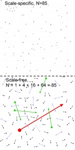
The illustration to the right (Figure 34 in my book) indicates the conceptual difference between classic and complex space use in terms of ergodicity. In this image consider – for the sake of model simplicity – that a population of 85 individuals (called an ensemble in statistical-mechanical jargon) are moving either “scale-specifically” (classic condition; upper panel) or “scale-free” (lower panel). The system is supposed to be closed; i.e., the individuals are bouncing back when reaching the borders of the available space. Consider that the respective individuals are located twice, and line segments are connecting the respective displacements. On one hand, consider that the chosen interval is chosen to be large enough to ensure that the “hidden layer” of unresolved path details is sufficiently deep to embed the necessary degrees of freedom (large number of unobserved micro-moves) to allow for a statistical-mechanical representation of the process. On the other hand, the interval is sufficiently small to make the probability of bounce-back from the area borders negligible during this interval of data collection. In other words, the system represents is closed, non-ergodic, and far from statistical-mechanical equilibrium at this time scale.
In the scale-specific case (upper panel), displacement vectors are not varying much; in a statistical analysis of move length they are in totality complying with a negative exponential distribution of displacements. This follows from the assumption of a scale-specific process and a sufficiently deep hidden layer (see the book for details). Under this condition, even totally deterministic movement below the hidden layer will appear stochastic and Brownian motion-like at our chosen temporal resolution for fix sampling. In contrast, consider the scale-free space-use variant in the lower panel, where some individuals have performed larger displacements during the interval. Specifically, in this scenario the distribution of displacement lengths complies statistically with a power law (may thus look like a Lévy walk) rather than an exponential at the given time resolution. The behavioural basis for the qualitative difference between the two scenaria is elaborated on in the book.
In the present context, just consider that the non-ergodic situation in the upper panel may be drifted towards an ergodic observation level on the system simply by decreasing the time resolution to allow for a high probability of intermediate border bounce-backs at this coarser time scale. However, the lower panel, representing complex space use, will require substantially larger time intervals to allow for ergodicity (technically, the Lévy walk-like process must reach the temporal limit for a transition towards Brownian motion; see Gautestad and Mysterud 2013).
With reference to the Scaling cube, the scenario in the upper panel catches the Brownian motion class of movement (lower left corner of the cube), under special condition of environmentally imposed constraint on area expansion (the convection model; the classic home range concept). The lower panel regards the upper left corner in the back of the cube, Levy walk, with a similar extrinsic constraint on free dispersal as in the first scenario. In the follow-up Part II of this post I elaborate on how an additional complexity-extended system description of these two scenaria may reveal properties that are counter-intuitive – in fact, paradoxical – from the classic perspective described above. The extra condition regards movement that is combined with site fidelity (occasional targeted returns to a previous location). In other words, we consider movement classes at the right-hand wall of the cube rather than the left-hand wall, where a home range emerges from intrinsic behaviour rather than extrinsic space use constraint.
These paradoxical properties to be elaborated on in Part II are in fact quite easy to verify in a set of GPS fixes, and under the extended theory the paradoxes are even resolved. However, a verification of complex space use makes traditional methods to calculate local habitat selection dubious.
Entropy is commonly understood as a measure of micro-scale particle disorder within a macroscopic system. This disorder; e.g., uncertainty with respect to a given particle’s exact location within a given time resolution, is quantified at a coarse scale of space and time. In other words, “the hidden layer” has to be sufficiently deep to allow for a simplified statistical-mechanical representation of the space use (see definition of the hidden layer in the post on the scaling cube). When the disorder is maximized, the system is in a state of equilibrium. In our context, the degree of “particle disorder” may be represented by a series of GPS relocations of an individual, and the “macroscopic” (or meso-scopic) aspect regards the statistical properties that emerge from the movement, which typically express some kind of area-constrained space use; i.e., a home range.
In traditional home range models, which come closest to classic statistical-mechanical system descriptions, the concept of entropy generally requires that…
- the macroscopic system is closed (i.e., spatially constrained movement), and the evolution of entropy regards how this property becomes maximized as the space use drifts towards equilibrium.
- In the context of a large set of GPS fixes under classically defined home range conditions, one might then assume the maximized entropy condition to be represented by serially non-autocorrelated fixes, as a result of applying a sufficiently large sampling interval between fixes. This condition supports system ergodicity. In mathematics, the term ergodic is used to describe a dynamical system which, broadly speaking, has the same behavior when averaged over time as averaged over the space of all the system’s states (phase space). In physics the term is used to imply that a system then satisfies the ergodic hypothesis of thermodynamics. (Wikipedia)
The illustration to the right (Figure 34 in my book) indicates the conceptual difference between classic and complex space use in terms of ergodicity. In this image consider – for the sake of model simplicity – that a population of 85 individuals (called an ensemble in statistical-mechanical jargon) are moving either “scale-specifically” (classic condition; upper panel) or “scale-free” (lower panel). The system is supposed to be closed; i.e., the individuals are bouncing back when reaching the borders of the available space. Consider that the respective individuals are located twice, and line segments are connecting the respective displacements. On one hand, consider that the chosen interval is chosen to be large enough to ensure that the “hidden layer” of unresolved path details is sufficiently deep to embed the necessary degrees of freedom (large number of unobserved micro-moves) to allow for a statistical-mechanical representation of the process. On the other hand, the interval is sufficiently small to make the probability of bounce-back from the area borders negligible during this interval of data collection. In other words, the system represents is closed, non-ergodic, and far from statistical-mechanical equilibrium at this time scale.
In the scale-specific case (upper panel), displacement vectors are not varying much; in a statistical analysis of move length they are in totality complying with a negative exponential distribution of displacements. This follows from the assumption of a scale-specific process and a sufficiently deep hidden layer (see the book for details). Under this condition, even totally deterministic movement below the hidden layer will appear stochastic and Brownian motion-like at our chosen temporal resolution for fix sampling. In contrast, consider the scale-free space-use variant in the lower panel, where some individuals have performed larger displacements during the interval. Specifically, in this scenario the distribution of displacement lengths complies statistically with a power law (may thus look like a Lévy walk) rather than an exponential at the given time resolution. The behavioural basis for the qualitative difference between the two scenaria is elaborated on in the book.
In the present context, just consider that the non-ergodic situation in the upper panel may be drifted towards an ergodic observation level on the system simply by decreasing the time resolution to allow for a high probability of intermediate border bounce-backs at this coarser time scale. However, the lower panel, representing complex space use, will require substantially larger time intervals to allow for ergodicity (technically, the Lévy walk-like process must reach the temporal limit for a transition towards Brownian motion; see Gautestad and Mysterud 2013).
With reference to the Scaling cube, the scenario in the upper panel catches the Brownian motion class of movement (lower left corner of the cube), under special condition of environmentally imposed constraint on area expansion (the convection model; the classic home range concept). The lower panel regards the upper left corner in the back of the cube, Levy walk, with a similar extrinsic constraint on free dispersal as in the first scenario. In the follow-up Part II of this post I elaborate on how an additional complexity-extended system description of these two scenaria may reveal properties that are counter-intuitive – in fact, paradoxical – from the classic perspective described above. The extra condition regards movement that is combined with site fidelity (occasional targeted returns to a previous location). In other words, we consider movement classes at the right-hand wall of the cube rather than the left-hand wall, where a home range emerges from intrinsic behaviour rather than extrinsic space use constraint.
These paradoxical properties to be elaborated on in Part II are in fact quite easy to verify in a set of GPS fixes, and under the extended theory the paradoxes are even resolved. However, a verification of complex space use makes traditional methods to calculate local habitat selection dubious.
Hence, this series of posts’ theoretical focus on statistical mechanics also points towards practical consequences for ecological inference based on space use data.
REFERENCES
Gautestad A. O and A. Mysterud. 2013. The Lévy flight foraging hypothesis: forgetting about memory may lead to false verification of Brownian motion. Movement Ecology. 2013;1:1-18
REFERENCES
Gautestad A. O and A. Mysterud. 2013. The Lévy flight foraging hypothesis: forgetting about memory may lead to false verification of Brownian motion. Movement Ecology. 2013;1:1-18