Homogeneous or Heterogeneous Environment?
When simulating animal space use – whether at the level of individuals or populations – some of the first conditions to define regard the attributes of the arena. The environment may be simple (homogeneous) or complicated (heterogeneous). As always the choice is a matter of weighing model simplicity against realism. However, another dimension of this choice is often overlooked. Animal space use is always a mixture of intrinsic and extrinsic driving forces. Thus, by simulating in a homogeneous environment one may to some extent disentangle these aspects by studying the intrinsic dynamics first and then – in follow up simulations – adding extrinsic variability.
This is an important point to stress, since simple models in homogeneous environment have occasionally been criticized for lack of realism.
As an example of how simplicity may contribute to important insight, consider traditional home range simulations (the convection model), observed at a statistical-mechanical temporal scale with sufficiently deep hidden layer (see definition in the post on the scaling cube). Convection regards a mixture of diffusion and advection. In a homogeneous environment the former will tend to disperse the animal homogeneously. On the other hand, advection will tend to force the spatial scatter of fixes into a smooth utilization distribution function, with higher density of fixes close to the defined centre of attraction.
In a homogeneous environment one has the opportunity to study the relative effects from these two intrinsic driving forces in isolation, by running scenaria with variation of parameters for diffusion versus advection strength (and actual formulation for each of them).
The results may look trivially simplistic, but they represent the important foundation for the next step: adding realism by introducing a heterogeneous habitat. In the convection model the output in the form of a multi-modal and complicated utilization distribution in a heterogeneous environment will be substantially easier to comprehend, given the background from the homogeneous condition. Start with the simple – move towards the more complicated. Albert Einstein said something like “Always simplify a model as far as possible – but not further“. Hence, to study intrinsic aspects of space use behaviour, use a homogeneous environment. Then move to heterogeneous conditions to find the optimal level of simplicity for this – more realistic – condition with respect to exploring model architecture for ecological inference in the given context of interest.
 With respect to the convection model for home range behavour, simulation in a homogeneous environment has little to offer. This condition has already been explored in great detail over so many years and in so many contexts that there are no more nuggets to find. Both the theory (diffusion, advection and traditional statistical mechanics) and specific model variants are solidly developed from the “intrinsic behaviour” perspective. Only added complicatedness (terms for behavioural responses to specific environmental conditions) may bring up new insight.
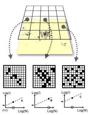
On the other hand, when it comes to complex space use, where intrinsic movement implies multi-scaled (and even scale-free) exploratory bouts of movement in parallel with spatial memory utilization (site fidelity), the theory is still in such an early phase of development that there is new insight to find around every corner. For example, the present illustration shows a simulated set of fixes from the MRW model, where the environment is conceptualized to be homogeneous in the centre and left part, and with lower quality in the rightmost part. The two left-hand sub-sections of the home range show how the individual’s characteristic scale of space use (CSSU) is of similar magnitude despite large difference in local density of fixes. CSSU is derived from the intercept with the y-axis in the Incidence regression log[I(N)].
These two localities have similar environmental conditions in the simulation; i.e, this part of the home range covers a homogeneous environment. The CSSU reveals this condition with great statistical clarity, while the classic density proxy N/A does not, given the present premise of complex space use.
On the other hand, the right-hand locality is in a lower-quality environment. The space use thus reflects this, by a larger y-intecept (larger CSSU, and thus weaker habitat selection strength in this locality), despite equal N in the leftmost and rightmost examples. In other words, the local density of fixes, N/A, is the same in the leftmost and rightmost analysis, but in the latter case N fixes are less “clumped” – more spatially randomomized – at the finer spatial resolution (smaller pixel size within the grid cell). Thus, incidence is larger for a given N.
This conceptual illustration exemplifies why my simulations of the MRW model typically have been executed in a homogeneous environment. For example, the CSSU concept was derived from this condition, and several theoretical predictions based on this condition were verified in follow-up simulations in heterogeneous environment. Several steps towards more realistic and heterogeneous scenaria have been performed, and more are in the coming.
This is an important point to stress, since simple models in homogeneous environment have occasionally been criticized for lack of realism.
As an example of how simplicity may contribute to important insight, consider traditional home range simulations (the convection model), observed at a statistical-mechanical temporal scale with sufficiently deep hidden layer (see definition in the post on the scaling cube). Convection regards a mixture of diffusion and advection. In a homogeneous environment the former will tend to disperse the animal homogeneously. On the other hand, advection will tend to force the spatial scatter of fixes into a smooth utilization distribution function, with higher density of fixes close to the defined centre of attraction.
In a homogeneous environment one has the opportunity to study the relative effects from these two intrinsic driving forces in isolation, by running scenaria with variation of parameters for diffusion versus advection strength (and actual formulation for each of them).
The results may look trivially simplistic, but they represent the important foundation for the next step: adding realism by introducing a heterogeneous habitat. In the convection model the output in the form of a multi-modal and complicated utilization distribution in a heterogeneous environment will be substantially easier to comprehend, given the background from the homogeneous condition. Start with the simple – move towards the more complicated. Albert Einstein said something like “Always simplify a model as far as possible – but not further“. Hence, to study intrinsic aspects of space use behaviour, use a homogeneous environment. Then move to heterogeneous conditions to find the optimal level of simplicity for this – more realistic – condition with respect to exploring model architecture for ecological inference in the given context of interest.
On the other hand, when it comes to complex space use, where intrinsic movement implies multi-scaled (and even scale-free) exploratory bouts of movement in parallel with spatial memory utilization (site fidelity), the theory is still in such an early phase of development that there is new insight to find around every corner. For example, the present illustration shows a simulated set of fixes from the MRW model, where the environment is conceptualized to be homogeneous in the centre and left part, and with lower quality in the rightmost part. The two left-hand sub-sections of the home range show how the individual’s characteristic scale of space use (CSSU) is of similar magnitude despite large difference in local density of fixes. CSSU is derived from the intercept with the y-axis in the Incidence regression log[I(N)].
These two localities have similar environmental conditions in the simulation; i.e, this part of the home range covers a homogeneous environment. The CSSU reveals this condition with great statistical clarity, while the classic density proxy N/A does not, given the present premise of complex space use.
On the other hand, the right-hand locality is in a lower-quality environment. The space use thus reflects this, by a larger y-intecept (larger CSSU, and thus weaker habitat selection strength in this locality), despite equal N in the leftmost and rightmost examples. In other words, the local density of fixes, N/A, is the same in the leftmost and rightmost analysis, but in the latter case N fixes are less “clumped” – more spatially randomomized – at the finer spatial resolution (smaller pixel size within the grid cell). Thus, incidence is larger for a given N.
This conceptual illustration exemplifies why my simulations of the MRW model typically have been executed in a homogeneous environment. For example, the CSSU concept was derived from this condition, and several theoretical predictions based on this condition were verified in follow-up simulations in heterogeneous environment. Several steps towards more realistic and heterogeneous scenaria have been performed, and more are in the coming.