MRW and Ecology – Part VI: The Statistical Property of Return Events
Animals that combine scale-free space use with targeted returns to previous locations generate a self-organized kind of home range. In short, the home range becomes an emergent property from such self-reinforcing revisits. Obviously, any space use pattern from complex processes outside the domain of Markov (mechanistic) theory needs to be analyzed using methods that are coherent with this kind of behaviour. Below I exemplify further the versatility of the MRW approach to adjust for serial auto-correlation (see Part III). I also show the quite surprising model property that the sub-set of inter-fix displacement lengths for return events seems to have a similar statistical distribution as the over-all pattern of exploratory step lengths. This additional emergent property of space use may lead to methods to test a wide range of behaviour-ecological hypotheses, for example to which extent an animal calculates on an energy cost with respect to distance to potential target locations for returns.
In ecological research it is traditionally considered logical that an animal considers a return to a distant familiar location to be less preferred than revisiting closer locations. On the other hand, by default (a priori) the MRW model does not include such a distance penalty on long-distance returns. Recently, the realism of this model premise has gained empirical support from studies on bison and toads (Merkle et al. 2014,2017; Marchand et al. 2017) (search Archive). In the MRW model’s standard version, a given return step is targeting any previous locations with equal probability except for the additive effect of number of previous visits to a given site, which increases the statistical probability for future revisits (self-reinforcing site fidelity). The implicit assumption is that the added energetic cost from long distance returns either is negligible relative to other parts of the energy budget, or the fitness value from keeping in touch with familiar locations regardless of current distance far exceeds the energy consideration. While this property regards a homogeneous environment it is trivial to adjust to a heterogeneous scenario without loss of the general principle. In this post I present more details on the return step property of MRW from a theoretical angle, as a starting point to test the model’s default condition on real data.
First, consider that the robustness of the MRW-based method to estimate an individual’s characteristic scale of space use (CSSU) within a given time and space extent is key to understand the energy aspect of return events as outlined above. The property of return events imposes a characteristic scale; i.e., CSSU, on space use, despite the scale-free nature of exploratory steps. For a given period, CSSU is a combined function of average movement speed and average return frequency. In a previous post I proposed how CSSU may be estimated even in auto-correlated (“over-sampled”) data series of location fixes. In this post I present a pilot analysis which strengthens this approach.
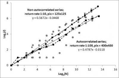 Consider the two simulated Home range ghost results to the right; incidence, I, as a function of number of fixes, N. The first set of fixes (circles) regards weakly auto-correlated series of fixes from return rate 1:10 and fix sampling at 1:100, while the second series (squares) resulted from a strongly autocorrelated path sampling (return rate 1:100 and sampling at 1:10). As was shown in Part III of this set of blog posts, by performing the “averaging trick” on log(I,N) from frequency and continuous sampling (open symbols for respective sets) the average log-log slope remains close to z = 0.5 (area expanding proportionally with square root of sample size) even for the strongly auto-correlated series. The slight deviance from z = 0.5 in the two series should be considered normal variability to be expected from one simulated series to the next (averaging over large sets of series would bring z closer to 0.5).
Critically, the present result also shows compliance with the expected change of the characteristic scale of space use (CSSU, represented by the parameter c in the Home range ghost formula I = cN0.5) as a function of the ratio between frequency of return events relative to exploratory moves (assuming constant average movement speed). In other words, observation frequency, which represents a sub-set of all displacements along a path (sampling of fixes) should not influence the CCSU estimate despite influencing the degree of auto-correlation. According to MRW theory, fewer returns during a constant average movement speed lead to larger CSSU*. In the analysis of the present two series, ten times smaller return rate led to an optimized unit pixel size (I ≡ 1) of magnitude √10 = 3.3 times larger than for the weakly autocorrelated series with higher return frequency.
In the Figure above, the two CSSU scales have both been rescaled to c = 1 ([log(c)=0], but respective series’ unit scale (I=1) is de facto correctly found to be very different in absolute terms.In the present examples, CSSU was estimated to c1 = 1252 area units for the high frequency return scenario and c2 = 4002 area units for the second series with fewer returns (and stronger degree of autocorrelation).
To conclude, after optimizing pixel size in respective series by analyzing I(N) over a range of pixel resolutions as previously described in my book and other posts, this preliminary analysis verifies a strong coherence between return step frequency and the magnitude of CSSU in accordance to the theoretical parameter prediction, despite strong difference in degree of serial autocorrelation in the sample of relocations. On other words, the CSSU estimate is quite resilient to the researcher’s choice of fix sampling scheme.
However, another aspect of the return step component of may turn out to be valuable to test the opposing energy hypotheses with respect to distance penalty, as outlined above.
Quite surprisingly I must admit, even considering the implicit “no distance penalty” model design, the tail part of the step length distribution of returns is quite similar to the tail of observed step lengths (fixes) that are sampled from the total series of steps!
The example series below with the weakest degree of auto-correlation (circles in the Figure above) shows similar functional form between the over-all distribution of binned step lengths [log(L); red circles below] and return distances (open symbols)**.
 As expected from the weakly autocorrelated series, the fit to the power law function with Levy exponent β=2 of the exploratory steps is showing a clear “hump” in the extreme part of the Log(L) distribution of fixes, due to influence from intermediate return events.
For the more strongly autocorrelated series with N=10,000 fixes from a total series of 100,000 steps and a lower return frequency 1:100 (Figure below) we see – as theoretically expected – a more subdued hump for the fixes, due to less influence from return events***. The hump would be even less pronounced if the fix sampling frequency had been even larger (Gautestad and Mysterud 2013; in particular Figure A2 in Supplementary material).
 Again the tail distribution of return lengths – where the total set of 1,000 events is shown as triangles – is similar to the the over-all distribution of fixes (1,000 first and 1,000 last of the N=10,000 fixes, shown as red and green circles). The median length for return steps is larger under this scenario (740 length units, versus 262) due to a ten times lower return frequency in relative terms. On the other hand, the median length for the actual set of fixes is strongly reduced as a consequence of the ten times larger fix sampling frequency.
To summarize, while the estimate of CSSU is quite resilient to fix sampling frequency, the (observed) median step length of fixes and (unobserved) length of return steps are influenced by fix sampling rate and return rate, respectively. Despite independence between the median length for observed series and hidden return lengths, both aspects of movement show a similar distribution of lengths.
Finally, what if the return step targets had not been set a priori to be independent on distance; i.e., by invoking distance penalty on return events? I have not tested this aspect yet in a modified MRW simulation model, but intuitively I predict the distribution of return steps to morph towards a negative exponential function rather than a power law, as in the exploratory kind of moves. As a consequence, the “hump” effect in the distribution of fixes should also be more subdued. Hence, by testing the difference in functional form of return steps and step lengths of observed fixes, one may have a method to test empirically the energy hypothesis that was outlined above.
The challenge, of course, is to develop a method to distinguish between exploratory moves and return events in empirical data. In simulation data it is simple to filter out the returns; in true space use data it is necessary to distinguish returns from path crossing by chance. More on this methodology in an upcoming post.
NOTES
*) Thus, the ratio returns/exploratory moves have a similar influence on CSSU as a change in average movement speed where the speed is expressed as the average staying time in a given grid cell. In Gautestad and Mysterud 2010, Eq. 4, we defined the expected length of step x, Lx, as a function of a scaling parameter for movement speed δ and fractal dimension of the path, d:
Lx = (δ[1 − Rnd]) − 1/d (Eq. 4)
where Rnd is a random number 0 ≤ Rnd < 1 and δ is a scaling parameter. In some sense δ may be interpreted as a parameter for expected staying time in a given patch, since larger δ implies smaller Lx and thus increased local fix contagion. Gautestad and Mysterud 2010, p2744
Thus, by defining the space use’s fractal dimension D as D ≡ d, we have the relationship with CSSU’s Home range ghost parameter, c, and movement speed:
c ∝ 1/√δ | D = 1 (Eq 5).
**) Due to a return step frequency of 1:10 and actual fix sampling frequency of 1:100, the total set of return events exceeds the fix sample by a factor of 10. Thus, I have compared the distribution of of return lengths from the early part of the simulated path (open squares) with return lengths towards the end of the path (open triangles), keeping both samples at same size as the set of observed fixes. Red circles in the Figure above represent 10,000 fixes from a total series of 1 million steps. When studying the first and the last part of the 100,000 hidden return steps specifically, their distribution looks indistinguishable from the series of “observed” fixes. Triangles show the result for the first 10,000 return events, and the squares show the result from the last 10,000 returns during the total of one million steps.
***) In this example where observation frequency exceeds the intrinsic return frequency by a factor of 10, the first and last part of the set of fixes (red and green circles, respectively) was used for comparison with the total set of return steps (open triangles).
REFERENCES
Gautestad, A. O., and I. Mysterud. 2010. Spatial memory, habitat auto-facilitation and the emergence of fractal home range patterns. Ecological Modelling 221:2741-2750.
Gautestad, A. O., and A. Mysterud. 2013. The Lévy flight foraging hypothesis: forgetting about memory may lead to false verification of Brownian motion. Movement Ecology 1:1-18.
Marchand, P, M. Boenke and D. M. Green. 2017. A stochastic movement model reproduces patterns of site fidelity and long-distance dispersal in a population of Fowler’s toads (Anaxyrus fowleri). Ecological Modelling 360:63–69.
Merkle, J. A., D. Fortin and J. M. Morales. 2014. A memory-based foraging tactic reveals an adaptive mechanism for restricted space use. Ecology Letters 17:924–931.
Merkle, J. A., J. R. Potts and D. Fortin. 2017. Energy benefits and emergent space use patterns of an empirically parameterized model of memory-based patch selection. Oikos 126:185–195
In ecological research it is traditionally considered logical that an animal considers a return to a distant familiar location to be less preferred than revisiting closer locations. On the other hand, by default (a priori) the MRW model does not include such a distance penalty on long-distance returns. Recently, the realism of this model premise has gained empirical support from studies on bison and toads (Merkle et al. 2014,2017; Marchand et al. 2017) (search Archive). In the MRW model’s standard version, a given return step is targeting any previous locations with equal probability except for the additive effect of number of previous visits to a given site, which increases the statistical probability for future revisits (self-reinforcing site fidelity). The implicit assumption is that the added energetic cost from long distance returns either is negligible relative to other parts of the energy budget, or the fitness value from keeping in touch with familiar locations regardless of current distance far exceeds the energy consideration. While this property regards a homogeneous environment it is trivial to adjust to a heterogeneous scenario without loss of the general principle. In this post I present more details on the return step property of MRW from a theoretical angle, as a starting point to test the model’s default condition on real data.
First, consider that the robustness of the MRW-based method to estimate an individual’s characteristic scale of space use (CSSU) within a given time and space extent is key to understand the energy aspect of return events as outlined above. The property of return events imposes a characteristic scale; i.e., CSSU, on space use, despite the scale-free nature of exploratory steps. For a given period, CSSU is a combined function of average movement speed and average return frequency. In a previous post I proposed how CSSU may be estimated even in auto-correlated (“over-sampled”) data series of location fixes. In this post I present a pilot analysis which strengthens this approach.

Critically, the present result also shows compliance with the expected change of the characteristic scale of space use (CSSU, represented by the parameter c in the Home range ghost formula I = cN0.5) as a function of the ratio between frequency of return events relative to exploratory moves (assuming constant average movement speed). In other words, observation frequency, which represents a sub-set of all displacements along a path (sampling of fixes) should not influence the CCSU estimate despite influencing the degree of auto-correlation. According to MRW theory, fewer returns during a constant average movement speed lead to larger CSSU*. In the analysis of the present two series, ten times smaller return rate led to an optimized unit pixel size (I ≡ 1) of magnitude √10 = 3.3 times larger than for the weakly autocorrelated series with higher return frequency.
In the Figure above, the two CSSU scales have both been rescaled to c = 1 ([log(c)=0], but respective series’ unit scale (I=1) is de facto correctly found to be very different in absolute terms.In the present examples, CSSU was estimated to c1 = 1252 area units for the high frequency return scenario and c2 = 4002 area units for the second series with fewer returns (and stronger degree of autocorrelation).
To conclude, after optimizing pixel size in respective series by analyzing I(N) over a range of pixel resolutions as previously described in my book and other posts, this preliminary analysis verifies a strong coherence between return step frequency and the magnitude of CSSU in accordance to the theoretical parameter prediction, despite strong difference in degree of serial autocorrelation in the sample of relocations. On other words, the CSSU estimate is quite resilient to the researcher’s choice of fix sampling scheme.
However, another aspect of the return step component of may turn out to be valuable to test the opposing energy hypotheses with respect to distance penalty, as outlined above.
Quite surprisingly I must admit, even considering the implicit “no distance penalty” model design, the tail part of the step length distribution of returns is quite similar to the tail of observed step lengths (fixes) that are sampled from the total series of steps!
The example series below with the weakest degree of auto-correlation (circles in the Figure above) shows similar functional form between the over-all distribution of binned step lengths [log(L); red circles below] and return distances (open symbols)**.

For the more strongly autocorrelated series with N=10,000 fixes from a total series of 100,000 steps and a lower return frequency 1:100 (Figure below) we see – as theoretically expected – a more subdued hump for the fixes, due to less influence from return events***. The hump would be even less pronounced if the fix sampling frequency had been even larger (Gautestad and Mysterud 2013; in particular Figure A2 in Supplementary material).

To summarize, while the estimate of CSSU is quite resilient to fix sampling frequency, the (observed) median step length of fixes and (unobserved) length of return steps are influenced by fix sampling rate and return rate, respectively. Despite independence between the median length for observed series and hidden return lengths, both aspects of movement show a similar distribution of lengths.
Finally, what if the return step targets had not been set a priori to be independent on distance; i.e., by invoking distance penalty on return events? I have not tested this aspect yet in a modified MRW simulation model, but intuitively I predict the distribution of return steps to morph towards a negative exponential function rather than a power law, as in the exploratory kind of moves. As a consequence, the “hump” effect in the distribution of fixes should also be more subdued. Hence, by testing the difference in functional form of return steps and step lengths of observed fixes, one may have a method to test empirically the energy hypothesis that was outlined above.
The challenge, of course, is to develop a method to distinguish between exploratory moves and return events in empirical data. In simulation data it is simple to filter out the returns; in true space use data it is necessary to distinguish returns from path crossing by chance. More on this methodology in an upcoming post.
NOTES
*) Thus, the ratio returns/exploratory moves have a similar influence on CSSU as a change in average movement speed where the speed is expressed as the average staying time in a given grid cell. In Gautestad and Mysterud 2010, Eq. 4, we defined the expected length of step x, Lx, as a function of a scaling parameter for movement speed δ and fractal dimension of the path, d:
Lx = (δ[1 − Rnd]) − 1/d (Eq. 4)
where Rnd is a random number 0 ≤ Rnd < 1 and δ is a scaling parameter. In some sense δ may be interpreted as a parameter for expected staying time in a given patch, since larger δ implies smaller Lx and thus increased local fix contagion. Gautestad and Mysterud 2010, p2744
Thus, by defining the space use’s fractal dimension D as D ≡ d, we have the relationship with CSSU’s Home range ghost parameter, c, and movement speed:
c ∝ 1/√δ | D = 1 (Eq 5).
**) Due to a return step frequency of 1:10 and actual fix sampling frequency of 1:100, the total set of return events exceeds the fix sample by a factor of 10. Thus, I have compared the distribution of of return lengths from the early part of the simulated path (open squares) with return lengths towards the end of the path (open triangles), keeping both samples at same size as the set of observed fixes. Red circles in the Figure above represent 10,000 fixes from a total series of 1 million steps. When studying the first and the last part of the 100,000 hidden return steps specifically, their distribution looks indistinguishable from the series of “observed” fixes. Triangles show the result for the first 10,000 return events, and the squares show the result from the last 10,000 returns during the total of one million steps.
***) In this example where observation frequency exceeds the intrinsic return frequency by a factor of 10, the first and last part of the set of fixes (red and green circles, respectively) was used for comparison with the total set of return steps (open triangles).
REFERENCES
Gautestad, A. O., and I. Mysterud. 2010. Spatial memory, habitat auto-facilitation and the emergence of fractal home range patterns. Ecological Modelling 221:2741-2750.
Gautestad, A. O., and A. Mysterud. 2013. The Lévy flight foraging hypothesis: forgetting about memory may lead to false verification of Brownian motion. Movement Ecology 1:1-18.
Marchand, P, M. Boenke and D. M. Green. 2017. A stochastic movement model reproduces patterns of site fidelity and long-distance dispersal in a population of Fowler’s toads (Anaxyrus fowleri). Ecological Modelling 360:63–69.
Merkle, J. A., D. Fortin and J. M. Morales. 2014. A memory-based foraging tactic reveals an adaptive mechanism for restricted space use. Ecology Letters 17:924–931.
Merkle, J. A., J. R. Potts and D. Fortin. 2017. Energy benefits and emergent space use patterns of an empirically parameterized model of memory-based patch selection. Oikos 126:185–195