MRW and Ecology- Part VII: Testing Habitat Familiarity
Consider having a series of GPS fixes, and you wonder if the individual was utilizing familiar space during your observation period – or started building site familiarity around the time when you started collecting data. Simulation studies of Multi-scaled random walk (MRW) shows how you may cast light on this important ecological aspect of space use.
First, you should of course test for compliance with the MRW assumptions, (a) site fidelity with no “distance penalty” on return events, (b) scale-free space use over the spatial range that is covered by your data, and (c) uniform space utilization on average over this scale range. One single test in the MRW Simulator, the A(N) regression, cast light on all these aspects. First, you seek to optimize pixel resolution for the analysis (estimating the Characteristic scale of space use, CSSU). Next, if you find “Home range ghost” compliance; i.e., incidence I expands proportionally with square root of sample size of fixes, your data supports (a) spatial memory utilization with no distance penalty due to sub-diffusive and non-asymptotic area expansion, (b) scale-free space use due to linearity of the log[I(N)] scatter plot, and (c) equal inter-scale weight of space use due to slope ≈ 0.5.
Supposing your data confirmed MRW, how to test for time-dependent strength of habitat familiarity? Consider the following simulation example, mimicking space use during a season and under constant environmental conditions.
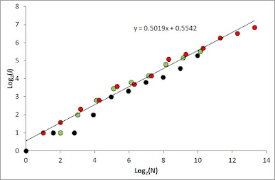 The red dots show log(N,I) for various sample sizes up to the total set of 11,000 fixes. Each dot represents the average I for respective N of the two methods continuous sampling and frequency sampling (counteracting autocorrelation effect; see a previous post). However, analyzing the first 1,000 fixes separately (black dots) consistently revealed a more sloppy space use in terms of aggregated incidence at a given N, relative to the total season. The next 1,000 fixes, however, was compliant with the total series both with respect to slope and y-intercept (CSSU) (green dots).
 The reason for the discrepancy in space use during the initial period of fix sampling* was in the present scenario the actual simulation condition; site familiarity was set to develop “from scratch” simultaneously with the onset of fix collection. I define strength of site familiarity as proportional with the total path length from which the model animal collects a previous location to return to**. In the start of the sampling period, the underlying path is short in comparison to the total path that was traversed during the total season, and – crucially – return steps targeted previous locations from the actual simulation period only, and not locations prior to to this start time. In other words, the animal was assumed to settle down in the area at the point in time when the simulation commenced.
To conclude, if your data shows CSSU and slope of similar magnitude in the early and later phase of data collection, you sampled an individual with a well-established memory map of its environment during the entire observation period. The implicit assumption for this conclusion is of course that the environmental conditions was constant during the entire sampling period, including the initial phase. Using empirical rather than synthetic data means that additional tests would have to be performed to cast light on this aspect.
NOTE
*) The presentation above reflects the pixel resolution that was optimized for the total series. The first 1,000 fixes showed a more coarse-grained space use, reflected in a 50% larger CSSU scale (not shown: optimal pixel size was 50% larger for this part of the series) despite constant movement speed and return rate for the entire simulation period. In this scenario a larger CSSU [coarser optimal pixel for the A(N) analysis] signals a less mature habitat utilization in the home range’s early phase. The CSSU was temporarily inflated during build-up of site familiarity, but – somewhat paradoxically – the accumulated number of fix-embedding grid cells (incidence) for a given N at this scale was smaller. These two effects, reflecting degree of habitat familiarity during home range establishment, should be considered a transient effect.
**) Two definitions should be specified:
First, you should of course test for compliance with the MRW assumptions, (a) site fidelity with no “distance penalty” on return events, (b) scale-free space use over the spatial range that is covered by your data, and (c) uniform space utilization on average over this scale range. One single test in the MRW Simulator, the A(N) regression, cast light on all these aspects. First, you seek to optimize pixel resolution for the analysis (estimating the Characteristic scale of space use, CSSU). Next, if you find “Home range ghost” compliance; i.e., incidence I expands proportionally with square root of sample size of fixes, your data supports (a) spatial memory utilization with no distance penalty due to sub-diffusive and non-asymptotic area expansion, (b) scale-free space use due to linearity of the log[I(N)] scatter plot, and (c) equal inter-scale weight of space use due to slope ≈ 0.5.
Supposing your data confirmed MRW, how to test for time-dependent strength of habitat familiarity? Consider the following simulation example, mimicking space use during a season and under constant environmental conditions.

To conclude, if your data shows CSSU and slope of similar magnitude in the early and later phase of data collection, you sampled an individual with a well-established memory map of its environment during the entire observation period. The implicit assumption for this conclusion is of course that the environmental conditions was constant during the entire sampling period, including the initial phase. Using empirical rather than synthetic data means that additional tests would have to be performed to cast light on this aspect.
NOTE
*) The presentation above reflects the pixel resolution that was optimized for the total series. The first 1,000 fixes showed a more coarse-grained space use, reflected in a 50% larger CSSU scale (not shown: optimal pixel size was 50% larger for this part of the series) despite constant movement speed and return rate for the entire simulation period. In this scenario a larger CSSU [coarser optimal pixel for the A(N) analysis] signals a less mature habitat utilization in the home range’s early phase. The CSSU was temporarily inflated during build-up of site familiarity, but – somewhat paradoxically – the accumulated number of fix-embedding grid cells (incidence) for a given N at this scale was smaller. These two effects, reflecting degree of habitat familiarity during home range establishment, should be considered a transient effect.
**) Two definitions should be specified:
- I define strength of site familiarity as proportional with the total path length from which the model animal collects a previous location to return to.
- I define strength of site fidelity as proportional with the return frequency. Both definitions rest on the assumptions of no distance penalty on return targets and no time penalty on returns; i.e., infinite spatio-temporal memory horizon relative to the actual sampling period.