The MRW Simulator: Importing Your Own GPS Data
You have a large database of GPS fixes, and you wonder if your animals have utilized their habitat in accordance to standard theory of mechanistic movement (the null hypothesis) or in compliance with the MRW theory (the alternative hypothesis). The MRW Simulator is tailormade for this kind of test. If MRW is verified you may proceed with various analyses of behavioural ecology under the alternative statistical-mechanical theory. The initial test procedure is simple: (1) import your data, (2) prepare for a test of model compliance by applying one or more built-in algorithms, and (3) import the generated data tables for statistical test into third party packages (R, Excel, etc.).
You can import data to the MRW Simulator by preparing a two-column text file, using comma or TAB as delimiter between the two coordinate values for successive locations.
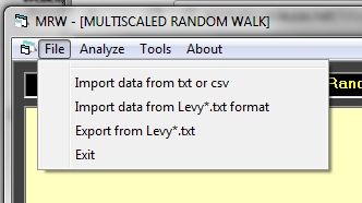 By default you should use the file name import.txt, but other names are also allowed (given the correct data structure). Place the file in the data folder (…/mov) and choose the menu “File | Import data from txt or csv”.
You are asked to define the file name for the imported data. By default, the name is set to “seed1.txt”. During importing the original series is centred on coordinate (0,0), the middle of the arena window. The arena size for the analysis is automatically adjusted to twice the space needed to display the set of the imported fixes.
After import, you set a couple of check boxes on the MRW Simulator’s user interface in accordance to User guide before clicking the run button (the MRW simulator re-formulates your imported data to its own format and saves the result in the text file levy1.txt). In particular, setting simulation series length to zero and choosing “use seed1.txt” as first part of the simulated series ensures that only your own data are reformatted. Within a fraction of a second the procedure exits without adding simulated data to the series, and you are ready to perform various analytical tasks on the levy1.txt file (see menu “Analyze”).
The procedure “A(N) regression” is typically applied to analyze space use at the home range scale. It is a convenient choice to test for MRW compliance of your data.
 You are asked which of the Levy*.txt files to analyze for fix-filling area as a function of sample size N (number of fixes in the Levy*.txt file). Next, the analysis is executed in accordance to the scales set in “Arena extent for analysis”, “Arena grain for analysis” and “Pixel (intra-grain resolution)” in the MRW Simulator’s user interface.
In this procedure, set extent = grain. Pixel regards a ratio; the relative resolution of grain/pixel. For example, setting pixel = 10 performs analysis at the virtual grid scale 1/10 of arena scale; i.e., 10×10 grid cells. See User guide for details.
The progress is shown below the arena window. The algorithm is counting incidence over a range of sample sizes N at the given pixel resolution; first by sequential (continuous) sampling up to Ntotal and then by frequency (uniform) sampling over the total series. Search my blog or read my book for these concepts.
 The result is saved in a text file containing a table of incidence (non-empty grid cells at the given pixel resolution) as a function of sample size N under the two sampling conditions. These data may then be imported in for example Excel for graphical presentation and statistical analysis; for example, a regression.
If you find a discrepancy between the scatter from the two sampling methods (you normally do!), your data is probably serially autocorrelated. To remove autocorrelation effect, take the average incidence for respective magnitudes of N, as was explained in a previous post. Conveniently, the MRW Simulator does this task for you (you find the averaging table below the tables for continuous and frequency sampling). This averaging procedure also adjusts for a “drifting home range” scenario, which also produces autocorrelation.
Does the result support MRW? First, you must verify presence of a characteristic scale of space use (CSSU), which is a property of scale-free movement under influence of spatial memory under the “parallel processing” postulate.
To test for CSSU you should experiment with various pixel resolutions and see if the log[(N,incidence)] pattern converges to a slope ∼0.5 at a given scale. If so, CSSU ≈ (pixel scale)2 = c.
If you don’t find reasonably good compliance with linearity of log[I(N)] = log(c) + 0.5*log(N) or the slope exceeds 0.5, try a coarser pixel resolution. If the slope is smaller than 0.5, try a finer pixel resolution.
If this test of convergence to log-linearity with slope ≈ 0.5 fails, you have probably either supported one of the null models; i.e., Brownian motion-like or Lévy-like space use void of spatial memory influence (slope ≈ 1, which is quite insensitive to change of pixel scale) or the classic paradigm: home range movement under influence of a constraining border zone [I(N) showing an area asymptote rather than a power law expansion with exponent close to 0.5].
The MRW Simulator 2.0 will now be made available as a free add-on tool for all buyers of my book. If you purchase it through my shopping cart at www.thescalingcube.com, you will get the program and its user guide bundled with the book. Existing book owners: contact me at arild@gautestad.com and I’ll fix you a personal download link – free of charge.
You can import data to the MRW Simulator by preparing a two-column text file, using comma or TAB as delimiter between the two coordinate values for successive locations.
You are asked to define the file name for the imported data. By default, the name is set to “seed1.txt”. During importing the original series is centred on coordinate (0,0), the middle of the arena window. The arena size for the analysis is automatically adjusted to twice the space needed to display the set of the imported fixes.
After import, you set a couple of check boxes on the MRW Simulator’s user interface in accordance to User guide before clicking the run button (the MRW simulator re-formulates your imported data to its own format and saves the result in the text file levy1.txt). In particular, setting simulation series length to zero and choosing “use seed1.txt” as first part of the simulated series ensures that only your own data are reformatted. Within a fraction of a second the procedure exits without adding simulated data to the series, and you are ready to perform various analytical tasks on the levy1.txt file (see menu “Analyze”).
The procedure “A(N) regression” is typically applied to analyze space use at the home range scale. It is a convenient choice to test for MRW compliance of your data.
In this procedure, set extent = grain. Pixel regards a ratio; the relative resolution of grain/pixel. For example, setting pixel = 10 performs analysis at the virtual grid scale 1/10 of arena scale; i.e., 10×10 grid cells. See User guide for details.
The progress is shown below the arena window. The algorithm is counting incidence over a range of sample sizes N at the given pixel resolution; first by sequential (continuous) sampling up to Ntotal and then by frequency (uniform) sampling over the total series. Search my blog or read my book for these concepts.
If you find a discrepancy between the scatter from the two sampling methods (you normally do!), your data is probably serially autocorrelated. To remove autocorrelation effect, take the average incidence for respective magnitudes of N, as was explained in a previous post. Conveniently, the MRW Simulator does this task for you (you find the averaging table below the tables for continuous and frequency sampling). This averaging procedure also adjusts for a “drifting home range” scenario, which also produces autocorrelation.
Does the result support MRW? First, you must verify presence of a characteristic scale of space use (CSSU), which is a property of scale-free movement under influence of spatial memory under the “parallel processing” postulate.
To test for CSSU you should experiment with various pixel resolutions and see if the log[(N,incidence)] pattern converges to a slope ∼0.5 at a given scale. If so, CSSU ≈ (pixel scale)2 = c.
If you don’t find reasonably good compliance with linearity of log[I(N)] = log(c) + 0.5*log(N) or the slope exceeds 0.5, try a coarser pixel resolution. If the slope is smaller than 0.5, try a finer pixel resolution.
If this test of convergence to log-linearity with slope ≈ 0.5 fails, you have probably either supported one of the null models; i.e., Brownian motion-like or Lévy-like space use void of spatial memory influence (slope ≈ 1, which is quite insensitive to change of pixel scale) or the classic paradigm: home range movement under influence of a constraining border zone [I(N) showing an area asymptote rather than a power law expansion with exponent close to 0.5].
The MRW Simulator 2.0 will now be made available as a free add-on tool for all buyers of my book. If you purchase it through my shopping cart at www.thescalingcube.com, you will get the program and its user guide bundled with the book. Existing book owners: contact me at arild@gautestad.com and I’ll fix you a personal download link – free of charge.