Animal Space Use

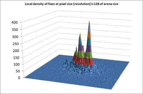
A growing number of analyses of spatial scatter of GPS positions of animals (fixes) verify a fractal dimension (D) substantially smaller than what should be expected from standard models. Specifically, D tends to be close to 1, which reflects a very heterogeneous fix dispersion over a wide range of spatial resolutions. A recurring question among analysts of animal space use is thus: is this so-called scale-free pattern – statistically speaking – reflecting a matching heterogeneous habitat that happens to satisfy a self-similar dispersion (the “environmental forcing” explanation), or is the scale-free space use a manifestation of intrinsic, cognitive processes (the “emergent property” explanation)? In this post I illustrate the challenge by showing an analysis of large mammals' space use. The image above, showing the spatial accumulation of fixes from GPS-sampling a red deer Cervus elaphus individual during the summer season illustrates this key question (see Gautestad et al. 2...

In my foregoing post I criticized the Burt legacy (Burt 1943) for hampering progress in analysis of animal space use on a local scale. Analyses of the spatial pattern of GPS fixes – when this has been explicitly explored by multi-scale methods – consistently confirm a statistical fractal with dimension 0.9 < D < 1.2 rather than a paradigm-confirming to-dimensional area demarcation (albeit with fuzzy borders; see below). In an ideal world the D≈1 result should lead to hefty follow-up tests from the community of animal ecologists for the sake of verifying or falsifying the “home range as a fractal”-model and its behavioural-ecological implications. After all, the home range concept is a cornerstone of animal ecology. Nope. The Burt legacy still appears impenetrable. However, things finally seem to start rolling. After a quarter of a century long invitation period following the initial papers on the topic (Loehle 1990; Gautestad and Mysterud 1993, 1994) the application of fractal...

The term “Home range” (HR) generally follows Burt’s (1943) definition, the area traversed by the individual in its normal activities of food gathering, mating, and caring for young. Occasional sallies outside of the area, perhaps exploratory in nature, should not be considered as home range. However, with respect to fine-grained perception of a HR, Burt’s definition seems to have guided – in fact cemented – the HR concept into a too narrow and partly misleading perception of individual space use. Hence, in my view the Burt definition is hampering progress in this important field of animal ecology. From the perspective of a regional map, an individual’s home range is a zero-dimensional dot. When zooming in towards medium scale, it makes sense to demarcate a home range as a two-dimensional area (or a three-dimensional volume in the context of aquatic or marine systems). The challenge to define HR borders at this scale is reflected in Burt’s second part of his HR definition, leaving som...

Time to verify theoretical coherence between scale-free population abundance and scale-free space use at the individual level! In this part IV of the Taylor law presentation I analyze a simulated set of GPS fixes rather than studying population abundance. In other words, how does the variance-mean relationship in local density of fixes from the multi-scaled random walk model (MRW) resemble V(M) in a local population under the Zoomer model condition? Through the history spanning more than 1,000 papers this acid test has never previously been successfully performed. My presentation also illustrates the so-called Z-paradox, and how it is resolved under the parallel processing framework for animal space use. The illustration to the right shows the spatial “home range” scatter from a model individual complying with the MRW model. The number of fixes pr. grid cell of resolution k=1:128 (128×128 cells within the defined arena) shows the commonly observed multi-modal utilization distrib...

Taylor’s power law regards the statistical relationship between population variance and population abundance, V = aM b . I refer to Parts I–II for background information. Whether V(M) is studied at a given spatial resolution or from varying abundance M in a sample by changing grid resolution the still unresolved problem is that animal populations (covering a wide range of taxa) upon re-scaling tend to show b≈2. Typical range is 1.5<≈b<≈2.2 rather than b≈1. In other words, due to the power law structure population dispersion seems to be scale-invariant; also called self-similar and thus compliant with a statistical fractal (aggregations within aggregations within…). In this post, I illustrate how V(M) in the Zoomer model becomes compliant with real-life V(M) patterns when the model is parameter-tuned towards its default condition – scale-free population dynamics! Many model proposals exist for V(M) when sampling at a given spatial resolution, but despite thousands of papers ov...

In a previous post I introduced the empirically observed Taylor’s power law, by referring to some of its history and one of its paradoxical properties: population abundance typically seems to satisfy a very aggregated pattern, V = aM b with b≈2, which seems to be self-similar (satisfying a statistical fractal) over a wide range of spatial resolutions. I also hinted towards chapters of my book, where I describe and discuss this and other strange statistical aspects relative to expectation from traditional population-dynamical models. In this post I study how my Zoomer model for scale-free population dynamics behave with respect to compliance with Taylor’s power law if I parameter-tune it towards more standard assumptions. Consider the generic statistical pattern that would be expected from a “well mixed” population (satisfying, for example the default assumption for a standard differential or difference equation model). In this case, which by the way also makes the model population...

A provocative headline is a double-edged sword. Why do I indicate that one of the most rapidly developing fields of animal ecology should still be regarded as a soft science? When it comes to individual space use rest assured that I’m thrilled by the substantial leaps forward in some parts of the theory of animal whereabouts. On the other hand, I also have critical comments. In my view there is still too strong disconnection between some general properties of movement-related animal behaviour and theoretical representations of this behaviour in models. Patch and resource sharing – butterfly Aglais io and bumblebee. Photo: AOG. Both in my book and in previous blog posts I have repeatedly pointed out the unfortunate fact that contemporary models in the field often referred to as “movement ecology” have matured into two quite distinct premise foundations. On one hand we see a broadened recognition of scale-free movement as a quite general property and on the other hand also a bro...