Animal Space Use

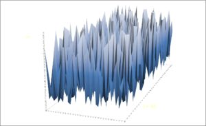
In the previous parts I-II of this series I described two variants of spatially extended population dynamics, represented by a standard Coupled map lattice (CML) model and the Zoomer model. In this post I show how a specific statistical-mechanical property of scale-free space use may reveal the difference between these two space use conditions despite an apparent similar level of spatial autocorrelation below the population’s carrying capacity. First, a brief summary of the model conditions (for details, see Part I-II): The environment is set to be homogeneous (be relaxed in upcoming posts), in order to have focus on intrinsic population kinetics.  The time resolution is set to be fine-grained, implying that the main driving force for change during respective time increments is individual re-shuffling rather than birth and death rates (net growth rate set to ca 1% in the present simulations).  For the CML examples (implying a scale-specific process in statistical-mechan...

In Part I of this series I presented spatially extended simulations of intrinsically driven population dynamics under the standard statistical-mechanical premises (intrinsically scale-specific), using a parsimonious Coupled map lattice (CML). In this Part II the framework will be extended with a scaling axis, orthogonal on space and time, to account for populations of individuals with space use satisfying the Multi-scaled random walk (MRW) properties. Using this scale-extended kind of CML design – the Zoomer model – I show how scale-free space use tend to generate spatial autocorrelation at the population level from conspecific attraction. The Zoomer model includes all the four standard BIDE rates (Birth, Immigration, Death and Emigration), and it is also spatially explicit. However, contrary to standard coupled map lattice models, spatial scale (the “lattice”) is implemented in a multi-scaled manner. This “scale range” approach allows for formulation of various aspects of complex p...

My book’s title reads: “Animal Space use: Memory Effects, Scaling Complexity, and Biophysical Model Coherence“. The latter part refers in particular to model compliance between individual- and population-level dynamics in spatially extended systems. Within the standard statistical-mechanical framework there is a well-developed theory for such coherence, based on memory-free and non-scaling (Markov-compliant) dynamics. However, as my book and blog is highlighting, the standard approaches towards modelling animal space use are often struggling when validated against high-quality spatio-temporal data. In a series of posts I illustrate challenges and potential solutions at the population level by exploring the Zoomer model – a parsimonious variant of the individual level Multi-scaled random walk model. First, I want to recap a citation from a previous post: “Parsimonious models are simple models with great explanatory predictive power. They explain data with a minimum number of paramet...

Focusing on the statistical pattern of space use without acknowledging the biophysical model for the process will create much confusion and unnecessary controversy. Ecologists are now forced to get a better grip on concepts from statistical mechanics than earlier generations. For example, to understand the transformation from data on actual behaviour to pattern analysis of space use, the concept of the hidden layer represents the first gate to pass. Research on animal movement and space use has always had a central place in ecology. However, as more field data, better computers and more sophisticated statistical methods have become available, some old dogma have come under attack. Specific theoretical aspects of this quest for improved model realism have emerged from the rapidly growing cooperation between biologists and physicists in the emerging field of macro-level biophysics. The so-called Lévy flight foraging hypothesis is one example. And, of course, I can’t resist mentioning t...

The default method to visualize a home range in the MRW Simulator is to just present the spatial scatter of fixes, without a traditional area demarcation. The scatter then represents a statistical fractal with properties to be explored by various methods. However, some kind of area demarcation has at least a visual appeal and may also be a necessity for some analytical purposes despite its intrinsic sample size dependency. Here I present a home range portrait that is based on an objective criterion from the MRW theory, the Characteristic scale of space use (CSSU). Using the CSSU scale [the unit spatial resolution when interpolating A(N, I ) to (1,1); i.e., “area per square root of N”] and superimposing a square of this size onto each fix in the series of N fixes is in my view a feasible choice. This alternative presentation of a home range outline should be applied after CSSU has been properly estimated using the A(N) regression method (for example, see this post). The text field “pi...

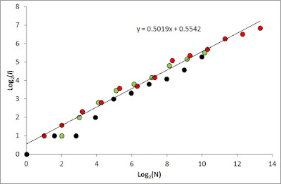
Consider having a series of GPS fixes, and you wonder if the individual was utilizing familiar space during your observation period – or started building site familiarity around the time when you started collecting data. Simulation studies of Multi-scaled random walk (MRW) shows how you may cast light on this important ecological aspect of space use. First, you should of course test for compliance with the MRW assumptions, (a) site fidelity with no “distance penalty” on return events, (b) scale-free space use over the spatial range that is covered by your data, and (c) uniform space utilization on average over this scale range. One single test in the MRW Simulator, the A(N) regression, cast light on all these aspects. First, you seek to optimize pixel resolution for the analysis (estimating the Characteristic scale of space use, CSSU). Next, if you find “Home range ghost” compliance; i.e., incidence I expands proportionally with square root of sample size of fixes, your data supports...

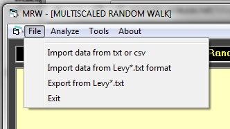
You have a large database of GPS fixes, and you wonder if your animals have utilized their habitat in accordance to standard theory of mechanistic movement (the null hypothesis) or in compliance with the MRW theory (the alternative hypothesis). The MRW Simulator is tailormade for this kind of test. If MRW is verified you may proceed with various analyses of behavioural ecology under the alternative statistical-mechanical theory. The initial test procedure is simple: (1) import your data, (2) prepare for a test of model compliance by applying one or more built-in algorithms, and (3) import the generated data tables for statistical test into third party packages (R, Excel, etc.). You can import data to the MRW Simulator by preparing a two-column text file, using comma or TAB as delimiter between the two coordinate values for successive locations. By default you should use the file name import.txt, but other names are also allowed (given the correct data structure). Place the file ...